Numpyro+jax based solution

M. Fouesneau¶

This Notebook shows how to implement a straight line fitting using MCMC and an outlier mixture model.

%%file requirements.txt
numpy
scipy
matplotlib
corner
daft
numpyro
funsor

Overwriting requirements.txt

#@title Install packages { display-mode: "form" }
# !pip install -r requirements.txt --quiet

#@title setup notebook { display-mode: "form" }
# Loading configuration
# Don't forget that mac has this annoying configuration that leads
# to limited number of figures/files
# ulimit -n 4096    <---- osx limits to 256

# Notebook matplotlib mode
%pylab inline                                 
# set for retina or hi-resolution displays
%config InlineBackend.figure_format='retina'  

light_minimal = {
    'font.family': 'serif',
    'font.size': 14,
    "axes.titlesize": "x-large",
    "axes.labelsize": "large",
    'axes.edgecolor': '#666666',
    "xtick.direction": "out",
    "ytick.direction": "out",
    "xtick.major.size": "8",
    "xtick.minor.size": "4",
    "ytick.major.size": "8",
    "ytick.minor.size": "4",
    'xtick.labelsize': 'small',
    'ytick.labelsize': 'small',
    'ytick.color': '#666666',
    'xtick.color': '#666666',
    'xtick.top': False,
    'ytick.right': False,
    'axes.spines.top': False,
    'axes.spines.right': False,
    'image.aspect': 'auto'
}

import pylab as plt
import numpy as np
plt.style.use(light_minimal)
from corner import corner
from IPython.display import display, Markdown

from itertools import cycle
from matplotlib.colors import is_color_like

def steppify(x, y):
    """ Steppify a curve (x,y). Useful for manually filling histograms """
    dx = 0.5 * (x[1:] + x[:-1])
    xx = np.zeros( 2 * len(dx), dtype=float)
    yy = np.zeros( 2 * len(y), dtype=float)
    xx[0::2], xx[1::2] = dx, dx
    yy[0::2], yy[1::2] = y, y
    xx = np.concatenate(([x[0] - (dx[0] - x[0])], xx, [x[-1] + (x[-1] - dx[-1])]))
    return xx, yy

def fast_violin(dataset, width=0.8, bins=None, color=None, which='both', 
                **kwargs):
    """ Make a violin plot with histograms instead of kde """
    
    if bins is None:
        a, b = np.nanmin(dataset), np.nanmax(dataset)
        d = np.nanstd(dataset, axis=0)
        d = np.nanmin(d[d>0])
        d /= np.sqrt(dataset.shape[1])
        bins = np.arange(a - 1.5 * d, b + 1.5 * d, d)
    
    default_colors = 'C0', 'C1', 'C2', 'C3', 'C4', 'C5', 'C6', 'C7', 'C8', 'C9'
    if is_color_like(color):
        colors = cycle([color])
    elif (color is None):
        colors = cycle(default_colors)
    elif len(color) != dataset.shape[1]:
        colors = cycle(default_colors)
    else:
        colors = color

    for k, color_ in zip(range(dataset.shape[1]), colors):
        n, bx = np.histogram(dataset[:, k], bins=bins, **kwargs)
        x_ = 0.5 * (bx[1:] + bx[:-1])
        y_ = n.astype(float) / n.max()
        y0_ = (k + 1) + np.zeros_like(x_)
        y1_ = (k + 1) + np.zeros_like(x_)
        if which in ('left', 'both'):
            y0_ += - 0.5 * width * y_
        if which in ('right', 'both'):
            y1_ += + 0.5 * width * y_

        r = plt.plot(y0_, x_, color=color_)
        plt.plot(y1_, x_, color=r[0].get_color())
        plt.fill_betweenx(x_, y0_, y1_,
                          color=r[0].get_color(), 
                          alpha=0.5)

        percs_where = np.array([0.16, 0.50, 0.84])
        percs_val = np.interp(percs_where, np.cumsum(y_) / np.sum(y_), x_)
        plt.plot([k + 1, k + 1], 
                 [percs_val[0], percs_val[2]], '-', color='k')
        plt.plot([k + 1], 
                 [percs_val[1]], 'o', color='k')

Populating the interactive namespace from numpy and matplotlib

Preliminary discussion around Bayesian statistics¶

As astronomers, we are interested in characterizing uncertainties as much as the point-estimate in our analyses. This means we want to infer the distribution of possible/plausible parameter values.

In the Bayesian context, the Bayes’ theorem, also called chain rule of conditional probabilities, expresses how a degree of belief (prior), expressed as a probability, should rationally change to account for the availability of related evidence.

P(A\mid B) = \frac{P(B \mid A) P(A)}{P(B)}

(1)

where $A$ and $B$ are ensembles of events. ( $P(B) \neq 0$ ).

$P(A\mid B)$ the probability of event $A$ occurring given that an event $B$ already occured. It is also called the posterior probability of $A$ given $B$ .
$P(B\mid A)$ is the probability of event $B$ occurring given that $A$ already occured. It is also called the likelihood of A given a fixed B.
$P(A)$ and $P(B)$ are the probabilities of observing $A$ and $B$ independently of the other one. They are known as the marginal probabilities or prior probabilities.

We note that in this equation we can swap $A$ and $B$ . The Bayesian framework only brings interpretations. One can see it as a knowledge refinement: given what I know about $A$ (e.g, gravity, stellar evolution, chemistry) what can we learn with new events $B$ .

A note about the proof: The equation derives from a simple observation (geometry/ensemble theory).

The figure below gives the visual support

#@title Baye's theorem figure { display-mode: "form" }
from matplotlib.patches import Ellipse, Rectangle

ax = plt.subplot(111)

patches = [
    Ellipse((-1, 0), 2, 3, angle=30, facecolor='0.5', edgecolor='k', alpha=0.1),
    Ellipse((-1, 0), 2, 3, angle=30, facecolor='None', edgecolor='k'),
    Ellipse((1, 0), 3, 2, angle=15, facecolor='0.5', edgecolor='k', alpha=0.1),
    Ellipse((1, 0), 3, 2, angle=15, facecolor='None', edgecolor='k'),
    Rectangle((-3, -3), 6, 6, facecolor='None', edgecolor='k')
]
for patch in patches:
    ax.add_patch(patch)
    
plt.text(-2.8, 2.8, r'$\Omega$', va='top', ha='left', color='k')
plt.text(-1, 0, 'A', va='top', ha='left', color='k')
plt.text(1, 0, 'B', va='top', ha='left', color='k')

plt.annotate(r'A$\cap$B', (-0.2, 0.), 
             xycoords='data',
             arrowprops=dict(facecolor='black', arrowstyle="->"),
             horizontalalignment='center', verticalalignment='bottom',
             xytext=(0.5, 1.5))

plt.xlim(-3, 3)
plt.ylim(-3, 3)

ax.get_xaxis().set_visible(False)
ax.get_yaxis().set_visible(False)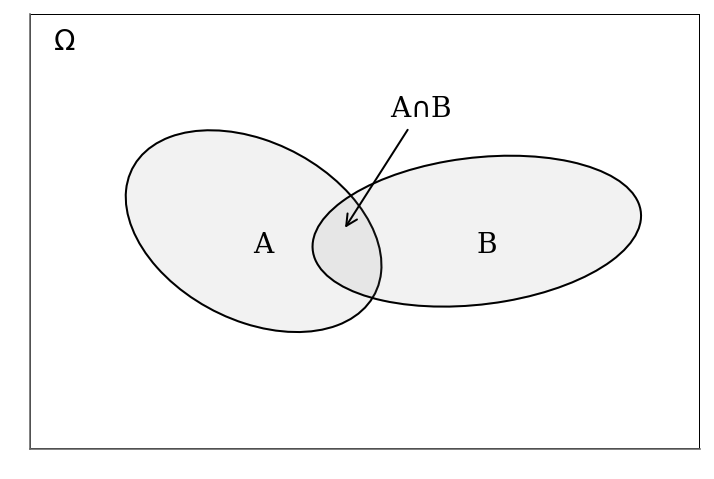

For any event $x$ from $\Omega$ $$

\begin{align*} P(x\in A \cap B) & = P(x\in A \mid x \in B) \cdot P(x\in B)\\ & = P(x\in B \mid x \in A) \cdot P(x\in A) \end{align*}

(2)

which we can write in a more compact way as

(3)

\begin{align*} P(A, B \mid \Omega) & = P(A \mid B, \Omega) \cdot P(B \mid \Omega)\\ & = P(B \mid A, \Omega) \cdot P(A \mid \Omega)\\ \end{align*}

(4)

$ $Note that, we explicitly noted$ \Omega$ but it is commonly omitted. The final equation of the Bayes’ theorem derives from the rearanging the terms of the right hand-side equalities.

The equation itself is most commonly attributed to reverand Thomas Bayes in 1763, but also to Pierre-Simon de Laplace. However, the current interpretation and usage significantly expanded from its initial formulation.

Straight line problem¶

In astronomy, we commonly have to fit a model to data. A very typical example is the fit of a straight line to a set of points in a two-dimensional plane. Astronomers are very good at finding a representation or a transformation of their data in which they can identify linear correlations (e.g., plotting in log-log space, action-angles for orbits, etc). Consequently, a polynomial remains a “line” in a more complicated representation space.

In this exercise, we consider a dataset with uncertainties along one axis only for simplicity, i.e. uncertainties along x negligible. These conditions are rarely met in practice but the principles remain similar. However, we also explore the outlier problem: bad data are very common in astronomy.

We emphasize the importance of having a “generative model” for the data, even an approximate one. Once there is a generative model, we have a direct computation of the likelihood of the parameters or the posterior probability distribution.

Problem definition¶

We will fit a linear model to a dataset $\{(x_i, y_i, \sigma_i)\}$

\hat{y}(x ~\mid~\alpha, \beta) = \alpha \cdot x + \beta.

(5)

Let’s start by looking at the data.

Generate dataset: Straight line with outliers¶

#@title Generate data { display-mode: "form" }
x = np.array([ 0,  3,  9, 14, 15, 19, 20, 21, 30, 35,
              40, 41, 42, 43, 54, 56, 67, 69, 72, 88])
y = np.array([33, 68, 34, 34, 37, 71, 37, 44, 48, 49,
              53, 49, 50, 48, 56, 60, 61, 63, 44, 71])
sy = np.array([ 3.6, 3.9, 2.6, 3.4, 3.8, 3.8, 2.2, 2.1, 2.3, 3.8,
               2.2, 2.8, 3.9, 3.1, 3.4, 2.6, 3.4, 3.7, 2.0, 3.5])

np.savetxt('line_outlier.dat', np.array([x, y, sy]).T)

x, y, sy = np.loadtxt('line_outlier.dat', unpack=True)
plt.errorbar(x, y, yerr=sy, marker='o', ls='None', ms=5, color='k');
plt.xlabel('X');
plt.ylabel('Y');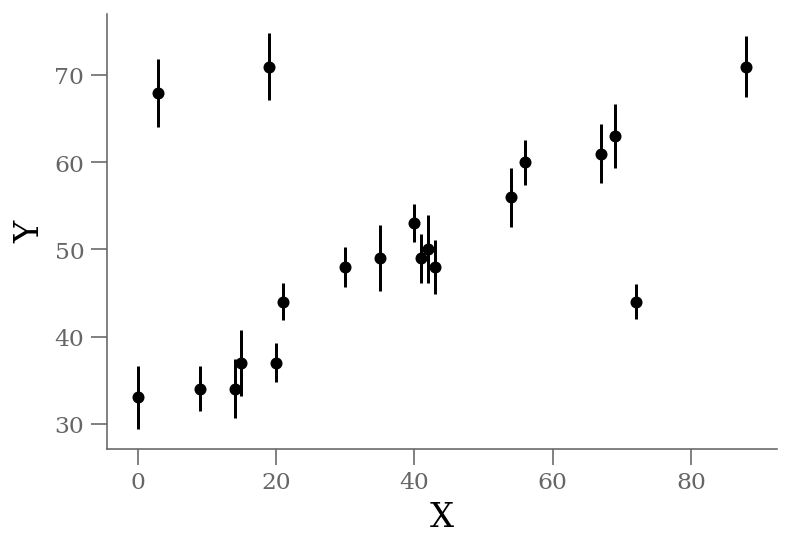

We see three outliers, but there is an obvious linear relation between the points overall.

Let’s see what happens if we fit the data without any outlier consideration.

Equations¶

We would like to fit a linear model to this above dataset:

\hat{y}(x ~\mid~\alpha, \beta) = \alpha x + \beta

(6)

We commonly start with the Bayes’s rule:

P(\alpha, \beta \mid \{x_i\}, \{y_i\}, \{\sigma_i\}) \propto P(\{x_i\}, \{y_i\} | \alpha, \beta, \{\sigma_i\}) P(\alpha, \beta)

(7)

Hence we need to define our prior and likelihood

Given this model and the gaussian uncertainties on our data, we can compute a Gaussian likelihood for each point:

P(x_i,y_i,~|~\alpha, \beta, \sigma_i) = \frac{1}{\sqrt{2\pi\sigma_i^2}} \exp\left[-\frac{1}{2\sigma_i^2}\left(y_i - {y}(x_i~|~\alpha, \beta)\right)^2\right]

(8)

Note that $\sigma_i$ is on the right hand side of the $\mid$ . It is because we assume given the Gaussian uncertainties when we write the likelihood that way.

The total likelihood is the product of all the individual likelihoods (as we assume independent measurements).

For numerical stability reasons, it is preferable to take the log-likelihood of the data. We have:

\log P(\{x_i, y_i\}~|~\alpha, \beta, \{\sigma_i\}) = \mathrm{const} - \sum_i \frac{1}{2\sigma_i^2}\left(y_i - y(x_i~|~\alpha, \beta)\right)^2

(9)

The posterior is the likelihood times the prior distributions. Let’s assume from the inspection of the data that $\alpha > 0$ , we can write

P(\alpha) = Uniform[0, 100],

(10)

and

P(\beta) = Uniform[0, 100].

(11)

(The upper value is abitrary.)

Coding¶

JAX is Autograd and XLA, brought together for high-performance machine learning research supported by Google.

Autograd: automatically differentiate native Python and NumPy functions. It can differentiate through loops, branches, recursion, and closures, and it can take derivatives of derivatives of derivatives. It supports reverse-mode differentiation (a.k.a. backpropagation) via grad as well as forward-mode differentiation, and the two can be composed arbitrarily to any order.

XLA: compile and run your NumPy programs on GPUs and TPUs. Compilation happens under the hood by default, with library calls getting just-in-time compiled and executed.

\begin{align*} \alpha &\sim \textrm{Uniform}(0, 100)\\ \beta &\sim \textrm{Uniform}(0, 100)\\ y_i &\sim \textrm{Normal}(\alpha \cdot x_i + \beta, \sigma_i) \end{align*}

(12)

import jax.numpy as jnp
from jax import random, vmap
from jax.scipy.special import logsumexp
import numpyro
from numpyro.diagnostics import hpdi
import numpyro.distributions as dist
from numpyro import handlers
from numpyro.infer import MCMC, NUTS

def jax_model_ols(x=None, y=None, sigma_y=None):
    beta = numpyro.sample("beta", dist.Uniform(0.0, 100))
    alpha = numpyro.sample("alpha", dist.Uniform(0.0, 100))
    ypred = beta + alpha * x
    numpyro.sample("y", dist.Normal(ypred, sigma_y), obs=y)

numpyro.render_model(jax_model_ols, model_args=(x, y, sy,), 
                     render_distributions=True)

Loading...

def jax_model_ols(x, y, sigma_y):
    beta = numpyro.sample("beta", dist.Normal(0.0, 100))
    alpha = numpyro.sample("alpha", dist.Normal(0.0, 100))
    with numpyro.plate("i=1..n", len(y)):
        ypred = beta + alpha * x
        numpyro.sample("y", dist.Normal(ypred, sigma_y), obs=y)

numpyro.render_model(jax_model_ols, model_args=(x, y, sy,),
                     render_distributions=True)

Loading...

# Start from this source of randomness. We will split keys for subsequent operations.
rng_key = random.PRNGKey(0)
rng_key, rng_key_ = random.split(rng_key)

# Run NUTS.
kernel = NUTS(jax_model_ols)
num_samples = 5000
mcmc = MCMC(kernel, num_warmup=3000, num_samples=num_samples)
mcmc.run(rng_key_, x=x, y=y, sigma_y=sy)
mcmc.print_summary()
traces_ols = mcmc.get_samples()

sample: 100%|██████████| 8000/8000 [00:09<00:00, 802.42it/s, 3 steps of size 3.93e-01. acc. prob=0.91]


                mean       std    median      5.0%     95.0%     n_eff     r_hat
     alpha      0.24      0.03      0.24      0.19      0.28   1312.33      1.00
      beta     39.68      1.24     39.68     37.64     41.77   1338.38      1.00

Number of divergences: 0

varnames = 'beta', 'alpha'
sample = np.array([traces_ols[k].ravel() for k in varnames]).T
corner(sample, labels=(r'$\beta$', r'$\alpha$'), quantiles=(0.16, 0.50, 0.84));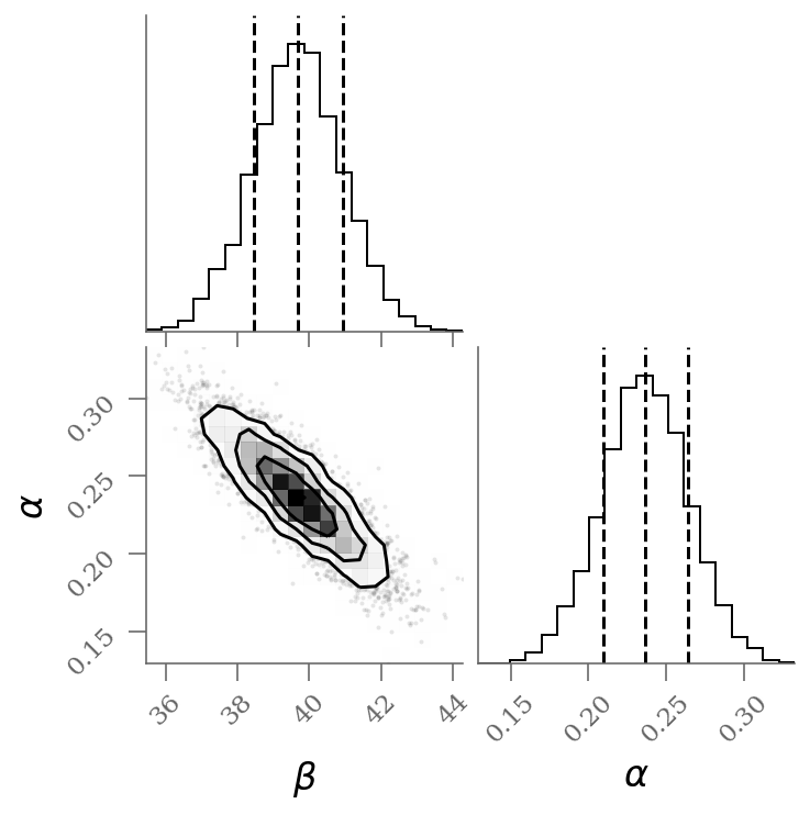

x, y, sy = np.loadtxt('line_outlier.dat', unpack=True)
plt.errorbar(x, y, yerr=sy, marker='o', ls='None', ms=5, color='k');
plt.xlabel('X');
plt.ylabel('Y');
ypred_blind = sample[:, 0] + sample[:, 1] * x[:, None]
plt.plot(x, ypred_blind[:, :100], color='C0', rasterized=True, alpha=0.3, lw=0.3)

percs_blind = np.percentile(sample, [16, 50, 84], axis=0)
display(Markdown(r"""Without outlier modeling:
* $\alpha$ = {1:0.3g} [{0:0.3g}, {2:0.3g}]
* $\beta$ = {4:0.3g} [{3:0.3g}, {5:0.3g}]
""".format(*percs_blind.T.ravel())
))

Loading...

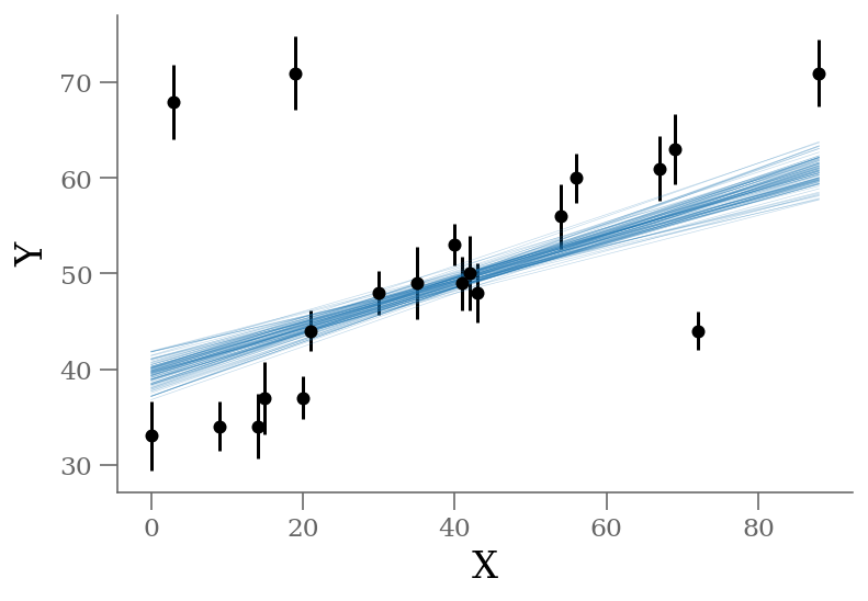
It’s clear from this plot that the outliers exerts a disproportionate influence on the fit.

This is due to the nature of our likelihood function. One outlier that is, say $10-\sigma$ (standard deviations) away from the fit will out-weight the contribution of points which are only $2-\sigma$ away.

In conclusion, least-square likelihoods are overly sensitive to outliers, and this is causing issues with our fit.

One way to address this is to simply model the outliers.

Mixture Model¶

The Bayesian approach to accounting for outliers generally involves mixture models so that the initial model is combined with a complement model accounting for the outliers:

P = q \cdot P_{in} + (1 - q) \cdot P_{out},

(13)

where $q$ is the mixing coefficient (between 0 and 1), $P_{in}$ and $P_{out}$ the probabilities of being an inlier and outlier, respectively.

So let’s propose a more complicated model that is a mixture between a signal and a background

Graphical model¶

A short parenthesis on probabilistic programming. One way to represent the above model is through probabilistic graphical models (pgm).

Using daft a python package, I draw a (inaccurate) pgm of the straight line model with outliers.

import daft

# Instantiate the PGM.
pgm = daft.PGM([4, 4], origin=[-0.5, -0.0], grid_unit=4, 
               node_unit=2, label_params=dict(fontsize='x-large'))

# Hierarchical parameters.
pgm.add_node(daft.Node("sout", r"$\sigma_{out}$", 0.9, 3.5, fixed=False))
pgm.add_node(daft.Node("g", r"$g$", 0.2, 3.5, fixed=False))
pgm.add_node(daft.Node("beta", r"$\beta$", 2.4, 3.5))
pgm.add_node(daft.Node("alpha", r"$\alpha$", 1.6, 3.5))

# Latent variable.
pgm.add_node(daft.Node("x", r"$x_i$", 1, 1))
pgm.add_node(daft.Node("gn", r"$g_i$", 0.2, 2, observed=False))
pgm.add_node(daft.Node("yin", r"$\hat{y}_{in}$", 2.5, 2, observed=False))
pgm.add_node(daft.Node("yout", r"$\hat{y}_{out}$", 1.5, 2, observed=False))

# Data.
pgm.add_node(daft.Node("y", r"$y_i$", 2, 1, observed=True))

# And a plate.
pgm.add_plate(daft.Plate([-0.2, 0.5, 3.2, 2.2], 
                         label=r"$i = 1, \cdots, N$", shift=-0.1,
                         bbox={"color": "none"}))

# add relations
pgm.add_edge("x", "y")
pgm.add_edge("alpha", "yin")
pgm.add_edge("beta", "yin")
pgm.add_edge("alpha", "yout")
pgm.add_edge("beta", "yout")
pgm.add_edge("sout", "yout")
pgm.add_edge("g", "gn")
pgm.add_edge("gn", "y")
pgm.add_edge("yin", "y")
pgm.add_edge("yout", "y")

pgm.render();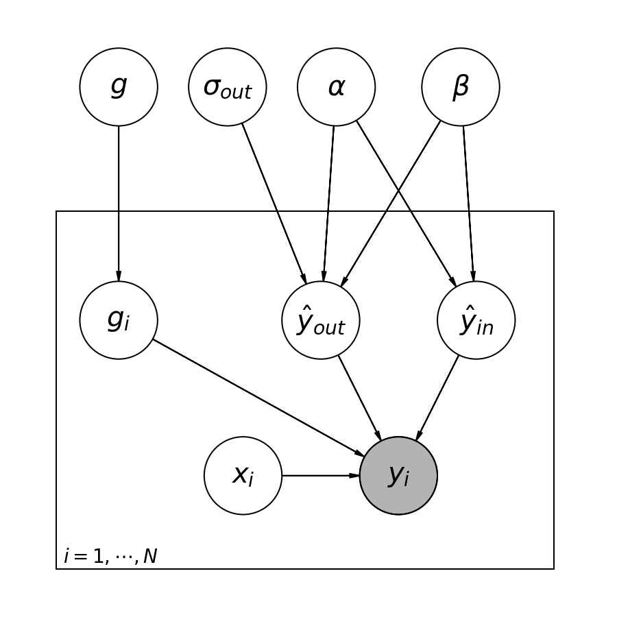

<Figure size 453.543x453.543 with 1 Axes>

There are multiple ways to define this mixture modeling.

Brutal version: 1 parameter per datapoint¶

P_i = q_i \cdot P_{in, i} + (1 - q_i) \cdot P_{out, i},

(14)

$P_{in, i}$ corresponds to the previous likelihood.

$P_{out, i}$ is arbitrary as we do not really have information about the causes for the outliers. We assume a similar Gaussian form centered on the affine relation but with a significantly larger dispersion. Doing so is intuitively considering the distance to the line to decide whether we have an outlier or not (this is intuitively a Bayesian version of sigma-clipping)

It is important to note that the total likelihood is a product of sums:

P = \prod_i P_i = \prod_i \left(q_i \cdot P_{in, i} + (1 - q_i) \cdot P_{out, i}\right).

(15)

Hence, we need to be careful to properly transform the $\ln P$ into $P$ during the calculations (see: np.logsumexp)

Hence the likelihood becomes explicitly

\begin{array}{ll} P(\{x_i\}, \{y_i\}~|~\theta,\{q_i\},\{\sigma_i\}, \sigma_{out}) = & \frac{q_i}{\sqrt{2\pi \sigma_i^2}}\exp\left[\frac{-\left(\hat{y}(x_i~|~\theta) - y_i\right)^2}{2\sigma_i^2}\right] \\ &+ \frac{1 - q_i}{\sqrt{2\pi \sigma_{out}^2}}\exp\left[\frac{-\left(\hat{y}(x_i~|~\theta) - y_i\right)^2}{2\sigma_{out}^2}\right]. \end{array}

(16)

We “simply” expanded our model with 20 nuisance parameters: $\{q_i\}$ is a series of weights, which range from 0 to 1 and encode for each point $i$ the degree to which it fits the model.

$q_i=0$ indicates an outlier, in which case a Gaussian of width $\sigma_{out}$ is used in the computation of the likelihood. This $\sigma_{out}$ can also be a nuisance parameter. However, for this example, we fix $\sigma_{out}$ to an arbitrary large value (large compared with the dispersion of the data)

Note that we have a prior that all $q_i$ must be strictly between 0 and 1.

We now make the probabilistic equations that link the various variables together:

We would like to fit a linear model to this above dataset:

\hat{y}_{in}(x ~\mid~\alpha, \beta) = \alpha x + \beta

(17)

One must provide some prior to properly implement the model. Let’s suppose weak informative normal priors (they correspond to a Ridge regression context)

\alpha \rightsquigarrow \mathcal{U}(0, 100)

(18)

\beta \rightsquigarrow \mathcal{U}(0, 100)

(19)

We also have the outlier component $\hat{y}_{out}$

\hat{y}_{out} \rightsquigarrow \mathcal{N}(\hat{y}_{out}, \sigma_{out})

(20)

where $\sigma_{out}$ is unknown but positively constrained (half-Normal prior)

\sigma_{out} \rightsquigarrow \mathcal{N^+}(0, 100)

(21)

And each data point has a probability (0 or 1) to be an outlier or not with a probability $g_i$

g_i \rightsquigarrow \mathcal{U}(0, 1)

(22)

(this is of course, sub-optimal)

Our final model is a mixture of the two components:

y_i ~\mid~ \hat{y}_{in}, \hat{y}_{out}, \sigma_y, \sigma_{out} \rightsquigarrow (1 - g_i) \, \mathcal{N}(\hat{y}_{in}, \sigma_y) + g_i \, \mathcal{N}(\hat{y}_{out}, \sigma_{out})

(23)

We code the model as:

def jax_model_brute(x=None, y=None, sigma_y=None):

    ## Define weakly informative Normal priors 
    beta = numpyro.sample("beta", dist.Uniform(0.0, 100))
    alpha = numpyro.sample("alpha", dist.Uniform(0.0, 100))

    ## variance of outliers
    sigma_y_out = numpyro.sample("sigma_y_out", dist.HalfNormal(100))

    ## model
    ypred = beta + alpha * x

    with numpyro.plate("i=1..n", len(y), dim=-1):
        ## define the linear model
        p_outlier = numpyro.sample('p_outlier', 
                                   dist.Uniform(0, 1))
        ## need a float for the mixture
        probs = jnp.stack([1 - p_outlier, p_outlier], axis=-1)

        locs_ = jnp.stack([ypred, ypred], -1)
        scales_ = jnp.stack([sigma_y, sigma_y_out * jnp.ones(len(x))], -1)
        comp_ = dist.Normal(locs_, scales_)
        mixture = dist.MixtureSameFamily(dist.Categorical(probs), comp_)

        # likelihood
        numpyro.sample("y", mixture, obs=y)

numpyro.render_model(jax_model_brute, model_args=(x, y, sy,),
                     render_distributions=True)

Loading...

# Start from this source of randomness. We will split keys for subsequent operations.
rng_key = random.PRNGKey(0)
rng_key, rng_key_ = random.split(rng_key)

# Run NUTS.
kernel = NUTS(jax_model_brute)
num_samples = 10_000
mcmc = MCMC(kernel, num_warmup=50_000, num_samples=num_samples)
mcmc.run(rng_key_, x=x, y=y, sigma_y=sy)
mcmc.print_summary()
traces = mcmc.get_samples()

sample: 100%|██████████| 60000/60000 [00:33<00:00, 1772.17it/s, 15 steps of size 3.20e-01. acc. prob=0.92]


                   mean       std    median      5.0%     95.0%     n_eff     r_hat
        alpha      0.46      0.04      0.46      0.39      0.53  10480.49      1.00
         beta     31.74      1.89     31.67     28.53     34.68  10084.71      1.00
 p_outlier[0]      0.38      0.26      0.34      0.00      0.78  19142.27      1.00
 p_outlier[1]      0.67      0.24      0.71      0.31      1.00  20917.21      1.00
 p_outlier[2]      0.38      0.27      0.34      0.00      0.79  16707.34      1.00
 p_outlier[3]      0.42      0.28      0.38      0.00      0.83  16934.32      1.00
 p_outlier[4]      0.39      0.27      0.35      0.00      0.79  18279.33      1.00
 p_outlier[5]      0.67      0.23      0.70      0.32      1.00  18118.53      1.00
 p_outlier[6]      0.45      0.29      0.42      0.00      0.87  16598.04      1.00
 p_outlier[7]      0.40      0.27      0.36      0.00      0.80  17744.98      1.00
 p_outlier[8]      0.39      0.27      0.34      0.00      0.79  20899.22      1.00
 p_outlier[9]      0.38      0.26      0.34      0.00      0.78  18410.61      1.00
p_outlier[10]      0.40      0.27      0.35      0.00      0.80  18262.61      1.00
p_outlier[11]      0.38      0.26      0.33      0.00      0.77  18054.81      1.00
p_outlier[12]      0.38      0.26      0.34      0.00      0.78  17200.75      1.00
p_outlier[13]      0.40      0.27      0.36      0.00      0.81  19761.69      1.00
p_outlier[14]      0.38      0.26      0.34      0.00      0.77  17896.72      1.00
p_outlier[15]      0.39      0.26      0.35      0.00      0.79  19058.08      1.00
p_outlier[16]      0.38      0.27      0.34      0.00      0.79  19299.24      1.00
p_outlier[17]      0.38      0.26      0.34      0.00      0.76  17660.67      1.00
p_outlier[18]      0.66      0.23      0.70      0.32      1.00  22792.29      1.00
p_outlier[19]      0.39      0.27      0.35      0.00      0.80  17606.22      1.00
  sigma_y_out     28.82     15.12     24.67     12.34     46.89   6879.70      1.00

Number of divergences: 0

varnames = 'beta', 'alpha', 'sigma_y_out'
sample = np.array([traces[k].ravel() for k in varnames]).T

corner(sample[:, :], labels=(r'$\beta$', r'$\alpha$', r'$\sigma_{out}$'), 
       quantiles=(0.16, 0.50, 0.84));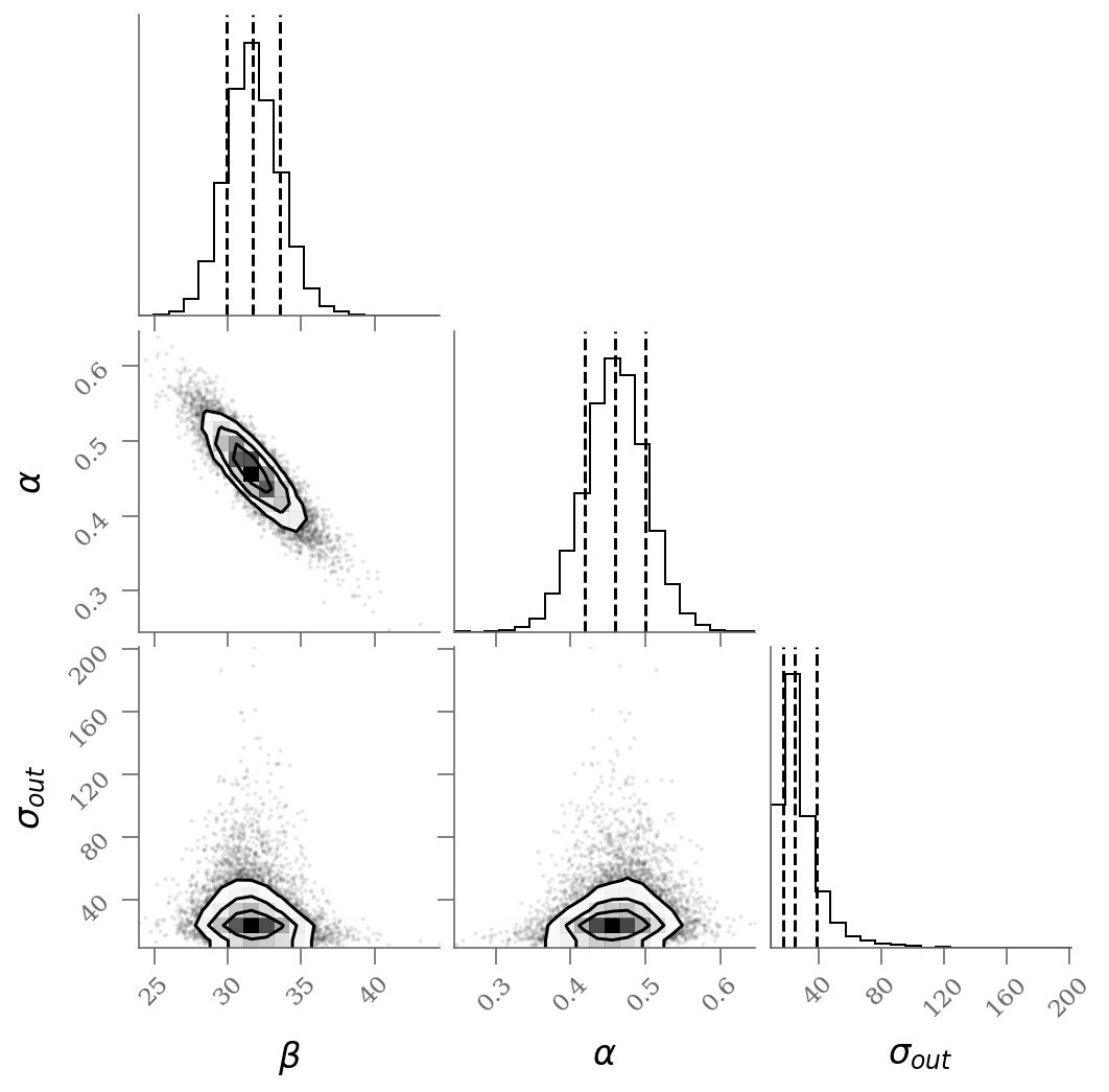

samples_q = 1 - traces['p_outlier'].T

plt.figure(figsize=(15, 5))
colors = np.where(np.median(samples_q, axis=1) < 0.5, 'C1', 'C0')
fast_violin(samples_q.T, color=colors)
ticks = (np.arange(samples_q.shape[0]) + 1)
lbls = [r'x$_{{{0:d}}}$'.format(k) for k in (0.5 * ticks).astype(int)]
plt.xticks(ticks, lbls)
plt.hlines([0.5], 0.5, len(ticks) + 0.5, color='0.5', zorder=-100, ls=':')
plt.xlim(0.5, len(ticks) + 0.5)
plt.ylabel('q_i');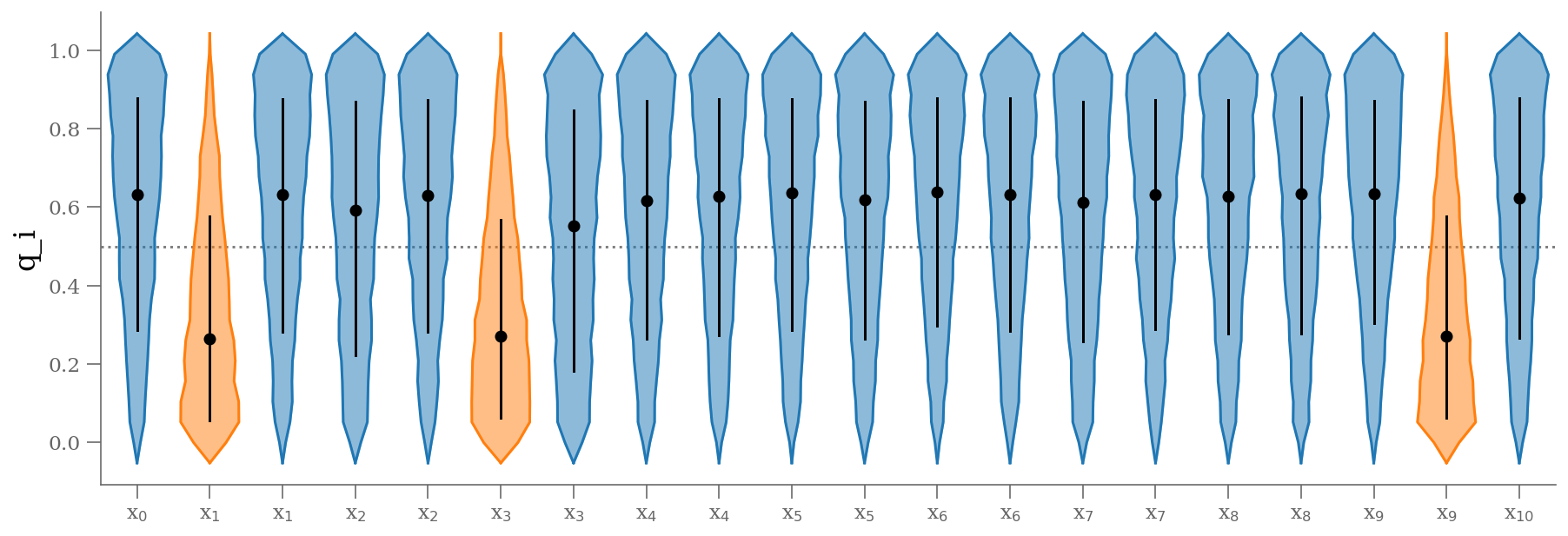

q = np.median(samples_q, 1)
outliers = (q <= 0.5)  # arbitrary choice
n_outliers = sum(outliers)

x, y, sy = np.loadtxt('line_outlier.dat', unpack=True)
plt.errorbar(x, y, yerr=sy, marker='o', ls='None', ms=5, color='k');
ypred_brute = sample[:, 0] + sample[:, 1] * x[:, None]

plt.plot(x, ypred_blind[:, :100], color='C0', rasterized=True, alpha=0.3, lw=0.3)
plt.plot(x, ypred_brute[:, :100], color='C1', rasterized=True, alpha=0.3, lw=0.3)
plt.plot(x[outliers], y[outliers], 'ro', 
         ms=20, mec='red', mfc='red', zorder=1, alpha=0.4)

plt.xlabel('X');
plt.ylabel('Y');


display(Markdown(r"""Without outlier modeling:
* $\alpha$ = {1:0.3g} [{0:0.3g}, {2:0.3g}]
* $\beta$ = {4:0.3g} [{3:0.3g}, {5:0.3g}]
""".format(*percs_blind.T.ravel())
))

percs_brute = np.percentile(sample[:, :2], [16, 50, 84], axis=0)
display(Markdown(r"""With outlier modeling: 22 parameters
* $\alpha$ = {1:0.3g} [{0:0.3g}, {2:0.3g}]
* $\beta$ = {4:0.3g} [{3:0.3g}, {5:0.3g}]
* number of outliers: ${6:d}$
""".format(*percs_brute.T.ravel(), n_outliers)
))

Loading...

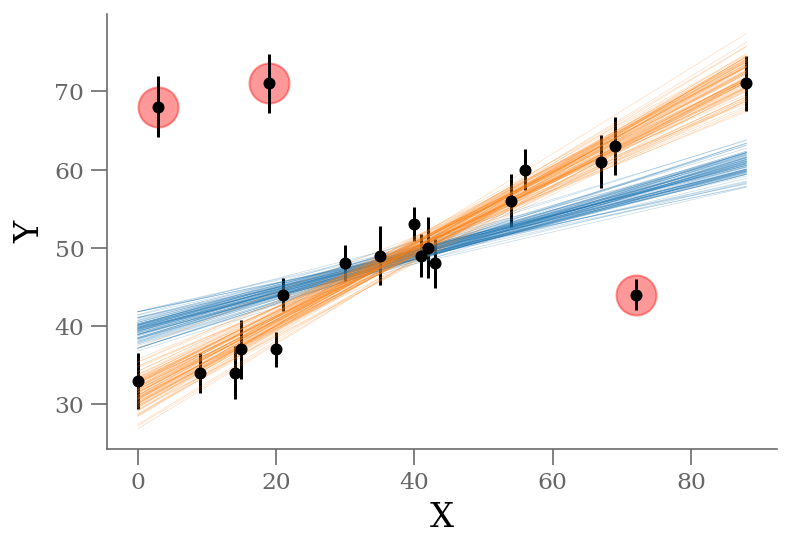
We see a distribution of points near a slope of $\sim 0.45$ , and an intercept of $\sim 31$ . We’ll plot this model over the data below, but first let’s see what other information we can extract from this trace.

One nice feature of analyzing MCMC samples is that the choice of nuisance parameters is completely irrelevant during the sampling.

The result shown in orange matches our intuition. In addition, the points automatically identified as outliers are the ones we would identify by eye to be suspicious. The blue shaded region indicates the previous “blind” result.

The smarter version¶

This previous model of outliers takes a simple linear model of 2 parameters and transforms it into a $(N+2)$ parameters, $N$ being the number of datapoints. This leads to 22 parameters in our case. What happens if you have 200 data points?

The problem with the previous model was that it adds one parameter for each data point, which not only makes the fitting expensive, but also makes the problem untracktable very quickly.

Based on the same formulation, we can consider one global $q$ instead individuals, which will characterize on the ensemble the probability of having an outlier. In other words, the fraction of outliers relative to the dataset.

P = \prod_i P_i = \prod_i \left(q \cdot P_{in, i} + (1 - q) \cdot P_{out, i}\right).

(24)

with

\begin{array}{ll} p(\{x_i\}, \{y_i\}~|~\theta,q,\{\sigma_i\}, \sigma_{out}) = & \frac{q}{\sqrt{2\pi \sigma_i^2}}\exp\left[\frac{-\left(\hat{y}(x_i~|~\theta) - y_i\right)^2}{2\sigma_i^2}\right] \\ &+ \frac{1 - q}{\sqrt{2\pi \sigma_{out}^2}}\exp\left[\frac{-\left(\hat{y}(x_i~|~\theta) - y_i\right)^2}{2\sigma_{out}^2}\right] \end{array}

(25)

We simply have 1 nuisance parameters: $q$ which ranges from 0 to 1.

Similarly to the previous model, $q=0$ indicates an outlier, in which case a Gaussian of width $\sigma_B$ is used in the computation of the likelihood. This $\sigma_B$ can also be a nuisance parameter.

From this model, we can estimate the odds of being an outlier with

Odds_{outlier}(x_i, y_i, \sigma_i) = \frac{(1-q) P(x_i, y_i | \sigma_{out})}{q\,P(x_i, y_i | \sigma_i, \alpha, \beta) + (1-q) P(x_i, y_i | \sigma_{out})}

(26)

Our likelihood can be expressed directly with tensor operations (otherwise we’d need to use theano’s @as_op decorator). This means we get the likelihood gradient for free thanks to the Theano backend, which makes the MCMC sampler more efficient (HMC methods)

We now make the probabilistic equations that link the various variables together:

We would like to fit a linear model to this above dataset:

\hat{y}_{in}(x ~\mid~\alpha, \beta) = \alpha x + \beta

(27)

One must provide some prior to properly implement the model. Let’s suppose weak informative normal priors (they correspond to a Ridge regression context)

\alpha \rightsquigarrow \mathcal{U}(0, 100)

(28)

\beta \rightsquigarrow \mathcal{U}(0, 100)

(29)

We also have the outlier component $\hat{y}_{out}$

\hat{y}_{out} \rightsquigarrow \mathcal{N}(\hat{y}_{out}, \sigma_{out})

(30)

where $\sigma_{out}$ is unknown but positively constrained (half-Normal prior)

\sigma_{out} \rightsquigarrow \mathcal{N^+}(0, 100)

(31)

$g$ sets the ratio of inliers to outliers. Given our setup, it corresponds to the fraction of outliers in our model. One can set a wealky informative prior on $g$ as

g \rightsquigarrow \mathcal{U}(0, 0.5)

(32)

(hopefully we do not have more than half of the data being made of outliers)

Our final model is a mixture of the two components:

y_i ~\mid~ \hat{y}_{in}, \hat{y}_{out}, \sigma_y, \sigma_{out} \rightsquigarrow (1 - g) \, \mathcal{N}(\hat{y}_{in}, \sigma_y) + g \, \mathcal{N}(\hat{y}_{out}, \sigma_{out})

(33)

we code the probabilistic model as follow (using DensityDist to set the final mixture likelihood)

def jax_model_outliers(x=None, y=None, sigma_y=None):

    ## Define weakly informative Normal priors 
    beta = numpyro.sample("beta", dist.Uniform(0.0, 100))
    alpha = numpyro.sample("alpha", dist.Uniform(0.0, 100))

    ## Define Bernoulli inlier / outlier flags according to 
    ## a hyperprior fraction of outliers, itself constrained
    ## to [0,.5] for symmetry
    frac_outliers = numpyro.sample('frac_outliers', 
                                   dist.Uniform(low=0., high=.5))

    ## variance of outliers
    sigma_y_out = numpyro.sample("sigma_y_out", dist.HalfNormal(100))

    # linear model
    ypred = beta + alpha * x
    
    # inliers
    ypred_in = dist.Normal(ypred, sigma_y)
    # ouliers
    ypred_out = dist.Normal(ypred, sigma_y_out)

    with numpyro.plate("i=1..n", len(y), dim=-1):
        ## define the linear model
        p_outlier = numpyro.sample('p_outlier', 
                                   dist.Bernoulli(frac_outliers), 
                                   infer={'enumerate': 'parallel'})
        
        ## need a float for the mixture
        probs = jnp.stack([1 - p_outlier, 
                           p_outlier], axis=-1).astype(float)

        locs_ = jnp.stack([ypred, ypred], -1)
        scales_ = jnp.stack([sigma_y_in  * jnp.ones(len(x)), 
                             sigma_y_out * jnp.ones(len(x))], -1)
        comp_ = dist.Normal(locs_, scales_)
        mixture = dist.MixtureSameFamily(dist.Categorical(probs), comp_)

        # calculate the outlier probability for book-keeping
        lnl_in = jnp.log(1 - frac_outliers) + ypred_in.log_prob(y)
        lnl_out = jnp.log(frac_outliers) + ypred_out.log_prob(y)
        ltot = jnp.logaddexp(lnl_in, lnl_out)
        q = numpyro.deterministic('q', jnp.exp(lnl_out) / jnp.exp(ltot))

        # likelihood
        numpyro.sample("y", mixture, obs=y)

numpyro.render_model(jax_model_outliers, model_args=(x, y, sy,),
                     render_distributions=True)

Loading...

# Start from this source of randomness. We will split keys for subsequent operations.
rng_key = random.PRNGKey(0)
rng_key, rng_key_ = random.split(rng_key)

# Run NUTS.
kernel = NUTS(jax_model_outliers)
num_samples = 5000
mcmc = MCMC(kernel, num_warmup=3000, num_samples=num_samples)
mcmc.run(rng_key_, x=x, y=y, sigma_y=sy)
mcmc.print_summary()
traces_smart = mcmc.get_samples()

sample: 100%|██████████| 8000/8000 [00:06<00:00, 1190.80it/s, 15 steps of size 3.48e-01. acc. prob=0.93]


                     mean       std    median      5.0%     95.0%     n_eff     r_hat
          alpha      0.47      0.04      0.47      0.41      0.53   2428.99      1.00
           beta     31.31      1.49     31.30     29.08     33.95   2394.69      1.00
  frac_outliers      0.21      0.09      0.20      0.06      0.36   2507.26      1.00
    sigma_y_out     41.06     22.91     34.93     14.32     69.36   2038.42      1.00

Number of divergences: 0

samples_q = 1 - traces_smart['q'].T

plt.figure(figsize=(15, 5))
colors = np.where(np.median(samples_q, axis=1) < 0.5, 'C1', 'C0')
fast_violin(samples_q.T, color=colors)
ticks = (np.arange(samples_q.shape[0]) + 1)
lbls = [r'x$_{{{0:d}}}$'.format(k) for k in (0.5 * ticks).astype(int)]
plt.xticks(ticks, lbls)
plt.hlines([0.5], 0.5, len(ticks) + 0.5, color='0.5', zorder=-100, ls=':')
plt.xlim(0.5, len(ticks) + 0.5)
plt.ylabel('q_i');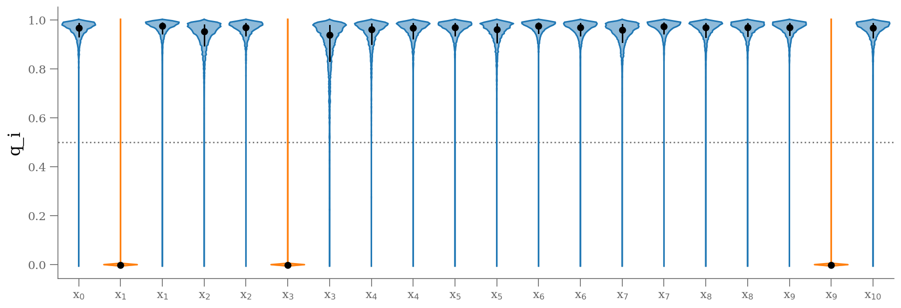

varnames = 'beta', 'alpha', 'frac_outliers', 'sigma_y_out'
sample = np.array([traces_smart[k].ravel() for k in varnames]).T

corner(sample[:, :], labels=(r'$\beta$', r'$\alpha$', r'1-q', r'$\sigma_{out}$'), quantiles=(0.16, 0.50, 0.84));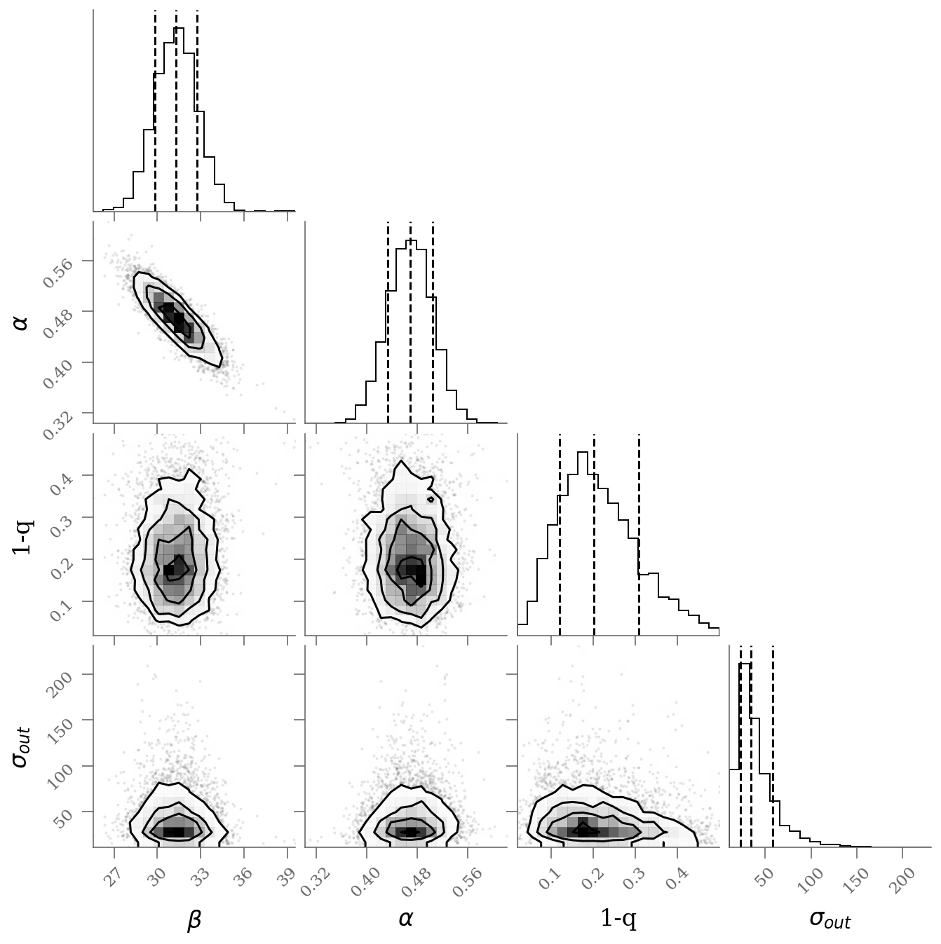

outliers = np.median(traces_smart['q'], axis=0) >= 0.5
n_outliers = int(sum(outliers))

x, y, sy = np.loadtxt('line_outlier.dat', unpack=True)
plt.errorbar(x, y, yerr=sy, marker='o', ls='None', ms=5, color='k');
ypred_smart = sample[:, 0] + sample[:, 1] * x[:, None]

plt.plot(x, ypred_blind[:, :100], color='C0', 
         rasterized=True, alpha=0.3, lw=0.3, zorder=-3)
plt.plot(x, ypred_brute[:, :1000], color='C1', 
         rasterized=True, alpha=0.3, lw=0.3, zorder=-2)
plt.plot(x, ypred_smart[:, :1000], color='C2', 
         rasterized=True, alpha=0.3, lw=0.3, zorder=-1)
plt.plot(x[outliers], y[outliers], 'ro', 
         ms=20, mec='red', mfc='red', zorder=1, alpha=0.4)

plt.xlabel('X');
plt.ylabel('Y');


display(Markdown(r"""Without outlier modeling (blue):
* $\alpha$ = {1:0.3g} [{0:0.3g}, {2:0.3g}]
* $\beta$ = {4:0.3g} [{3:0.3g}, {5:0.3g}]
""".format(*percs_blind.T.ravel())
))

display(Markdown(r"""With outlier modeling (orange): 22 parameters
* $\alpha$ = {1:0.3g} [{0:0.3g}, {2:0.3g}]
* $\beta$ = {4:0.3g} [{3:0.3g}, {5:0.3g}]
* number of outliers: ${6:d}$
""".format(*percs_brute.T.ravel(), n_outliers)
))

percs_smart = np.percentile(sample[:, :-1], [16, 50, 84], axis=0)
display(Markdown(r"""With outlier modeling (green): 3 parameters
* $\alpha$ = {1:0.3g} [{0:0.3g}, {2:0.3g}]
* $\beta$ = {4:0.3g} [{3:0.3g}, {5:0.3g}]
* $q$ = {7:0.3g} [{6:0.3g}, {8:0.3g}]
* number of outliers: ${9:d}$
""".format(*percs_smart.T.ravel(), n_outliers)
))

Loading...

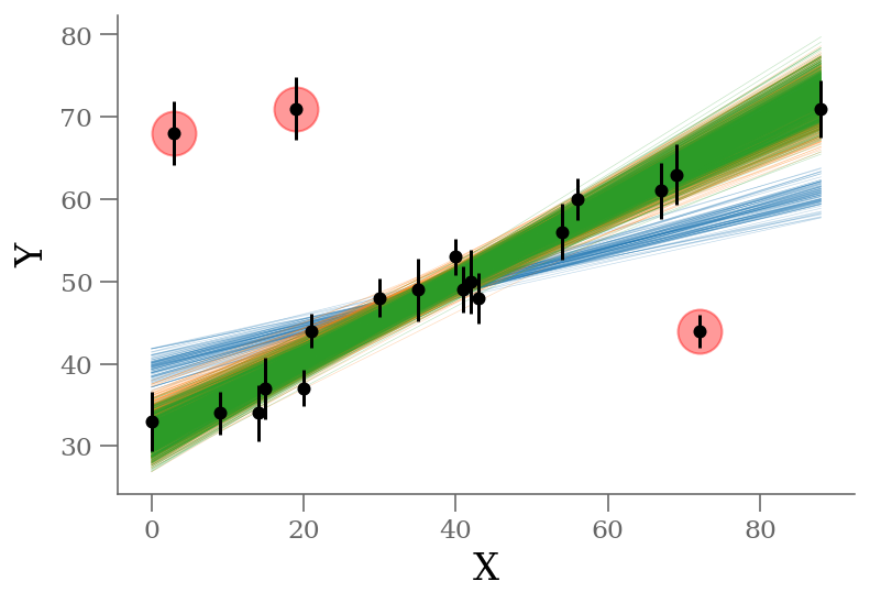
The infered parameters are nearly identical but the convergence is much faster in the last approach.

M. Fouesneau¶

Preliminary discussion around Bayesian statistics¶

Straight line problem¶

Problem definition¶

Generate dataset: Straight line with outliers¶

Blind fit: no outlier model¶

Equations¶

Coding¶

Mixture Model¶

Graphical model¶

Brutal version: 1 parameter per datapoint¶

The smarter version¶