This Notebook is part of the Workshop we gave at MPIA to introduce machine learning.
Setup project environement
First, we define a virtual environment for our project. This is a good practice to avoid conflicts between different projects. Details on how to create a virtual environment can be found on our FAQ here
Once done, we can activate the environment and install the required packages. We will use the following packages (for both days):
%%file requirements.txt

matplotlib
pandas
numpy
scikit-learn
torch
astropy
shap
tqdm
ipywidgets
requests
Overwriting requirements.txt
You can install the packages using the following command (after activating your virtual environment):
python3 -m pip install -q -r requirements.txtSetup notebook
%matplotlib inline
import pandas as pd
import numpy as np
import pylab as plt
# The following is only for the presentation, you can ignore it
from IPython.display import Markdown, display
plt.style.use('fivethirtyeight')
# to keep everything reproducible
np.random.seed(2024)
Introduction
In this notebook, we will introduce the basic concepts of machine learning and how to use Python to perform simple machine learning tasks.
This year, we will define concept throughout the entire workshop. We will start with the basic concepts and build on them as we go along.
Our project: Predicting galaxy redshift via regression on 3D-HST photometry
We will explore a typical machine learning problem: predicting galaxy redshifts from photometry. We will use the 3D-HST survey photometry to predict the redshift of galaxies.
The 3D-HST survey is a Hubble Space Telescope Treasury program that has used 248 orbits of HST time to image four fields in the sky with grism spectroscopy (AEGIS, COSMOS, GOODS-S, UKIDSS-UDS). See Brammer et al., 2012 and the 3D-HST website for more information.
The data we will use is a subset of the 3D-HST photometry and redshifts. We will use the photometry in the F125W, F140W, F160W, F606W, F814W filters, and the redshifts from the 3D-HST catalog from Skelton et al (2014).
Reminder Redshift 101
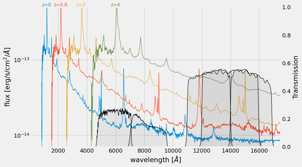
The redshift of a galaxy is a measure of how much the wavelength of light from the galaxy has been stretched by the expansion of the Universe. The redshift is defined as
where is the observed wavelength of light from the galaxy and is the wavelength of the light emitted by the galaxy.
Because of the spectrum shifts, an identical source at different redshifts will have a different color through each pair of filters.
from io import BytesIO
import requests
from astropy.io import votable


def get_svo_filter_profile(identifier: str) -> np.array:
    QUERY_URL = "http://svo2.cab.inta-csic.es/theory/fps/fps.php"
    query = {"ID": identifier}
    response = requests.get(QUERY_URL, params=query)
    response.raise_for_status()
    table = votable.parse_single_table(BytesIO(response.content))
    tab = table.to_table()
    return (tab["Wavelength"].to("angstrom").value, tab["Transmission"].data)
/Users/fouesneau/Work/projects/dsg_workshops/.venv/lib/python3.9/site-packages/urllib3/__init__.py:35: NotOpenSSLWarning: urllib3 v2 only supports OpenSSL 1.1.1+, currently the 'ssl' module is compiled with 'LibreSSL 2.8.3'. See: https://github.com/urllib3/urllib3/issues/3020
warnings.warn(
from astropy.io import fits

template_url = "https://archive.stsci.edu/hlsps/reference-atlases/cdbs/grid/comp_qso/optical_nir_qso_sed_001.fits"
with fits.open(template_url) as hdu:
    wave = hdu[1].data["WAVELENGTH"]
    flux = hdu[1].data["FLUX"]

plt.figure(figsize=(10, 6))

for z in (0, 0.8, 2, 4):
    line_color = plt.semilogy(wave * (1 + z), flux, lw=1)[0].get_color()
    plt.text(
        1_200 * (1 + z),
        5e-13,
        f"z={z}",
        ha="center",
        va="bottom",
        color=line_color,
        fontsize="small",
    )

plt.ylim(7e-15, 5e-13)
plt.xlim(86, 17_500)
plt.xlabel("wavelength [$\AA$]")
plt.ylabel("flux [erg/s/cm$^2$/$\AA$]")

ax = plt.twinx()
which_filters = [
    "HST/ACS_HRC.F606W",
    "HST/ACS_HRC.F814W",
    "HST/WFC3_IR.F125W",
    "HST/WFC3_IR.F140W",
    "HST/WFC3_IR.F160W",
]
for fname in which_filters:
    wave, trans = get_svo_filter_profile(fname)
    ax.plot(wave, trans, color="black", lw=1, label=fname)
    ax.fill_between(wave, trans, color="k", alpha=0.05)
    ax.set_ylim(0, 1)
    ax.grid(False)
ax.set_ylabel("Transmission")

Markdown("""
> **Figure**: Quasar template from [Glikman et al. 2006](https://ui.adsabs.harvard.edu/abs/2006ApJ...640..579G/abstract), and passbands from [The SVO Filter Profile Service](http://svo2.cab.inta-csic.es/theory/fps/) ([Rodrigo, C., Solano, E., 2020](https://ui.adsabs.harvard.edu/abs/2020sea..confE.182R/abstract))
""")
Download the data
First, we download the 3D-HST catalog from the MAST archive. Skelton et. al 2014 describe this dataset in details, especially the data selection.
from astropy.utils.data import download_file
import tarfile

file_url = "https://archive.stsci.edu/missions/hlsp/3d-hst/RELEASE_V4.0/Photometry/3dhst_master.phot.v4.1.tar"
tarfile.open(download_file(file_url, cache=True), "r:").extract(
    "3dhst_master.phot.v4.1/3dhst_master.phot.v4.1.cat", "."
)
Once we have the data on disk, we need to read the combined photmetric catalog.
Here is the first few lines of the file
# id field ra dec x y z_spec z_peak faper_F140W eaper_F140W faper_F160W eaper_F160W f_F606W e_F606W f_F814W e_F814W f_F125W e_F125W f_F140W e_F140W f_F160W e_F160W tot_cor kron_radius a_image b_image flux_radius fwhm_image flags f140w_flag star_flag use_phot near_star nexp_f125w nexp_f140w nexp_f160w lmass Av
# By K.E. Whitaker (3/14/2014)
    1.   AEGIS  215.22238159   53.00418472   9590.50   3057.30   -1.0000    0.0100 -8.2041E+01 -8.2041E+01  2.2531E+04  3.9282E-02  1.7906E+03  3.7991E-02  2.8049E+03  5.7433E-02  2.5063E+04  6.0967E-02 -9.9000E+01 -9.9000E+01  2.7188E+04  3.2896E-01    1.0088    3.5000      9.6500      8.8200    2.59E+00    3.4200   0   0   1   0   0   2   0   3    7.51   1.1
    2.   AEGIS  215.09658813   52.91805267  16473.20   3150.20   -1.0000    0.0100  3.5078E+00  7.4233E-02  3.9905E+00  3.7441E-02  9.0928E+01  1.7795E+00  1.4605E+02  2.7091E+00  2.5244E+02  3.0231E+00  2.5959E+02  5.4934E+00  2.9531E+02  1.6266E+00    1.0000    4.0800     31.1300     26.8900    3.81E+01   67.5200   3   0   0   0   0   4   4   4    5.62   0.1
Because the catalog is in ASCII format, we can use astropy and convert the Table into a pandas.dataframe object. The latter is more convenient with sklearn but cannot directly read the ASCII table (it contains misplaced comments).
from astropy.table import Table

df = Table.read(
    "3dhst_master.phot.v4.1/3dhst_master.phot.v4.1.cat", format="ascii"
).to_pandas()
For completeness, I show below how to directly read the file with pandas, but we need to deal with the misplaced comments.
# read the column header
with open("./3dhst_master.phot.v4.1/3dhst_master.phot.v4.1.cat") as f:
    header = f.readline().replace("#", "").split()
df = pd.read_csv(
    "./3dhst_master.phot.v4.1/3dhst_master.phot.v4.1.cat",
    sep="\s+",
    comment="#",
    names=header,
)
dfExploring the dataset
This section aims to examine the contents of the catalog.
The dataset contains standard information such as target id, field name, coordinates (ra, dec), fluxes, uncertainties, and various photometric flags (see Skelton et. al 2014 - Table 10, or download the README here).
In addition, there are some derived properties such as photometric redshift (z_peak), spectroscopic redshift (z_spec), mass (lmass) and dust extinction in the V band (Av).
Kriek et al (2018; FAST) describe the mass estimates.
Keep in mind that we are interested in predicting redshift, so our “target” variable will be z_spec. The “features” will be all relevant columns.
df.columnsIndex(['id', 'field', 'ra', 'dec', 'x', 'y', 'z_spec', 'z_peak', 'faper_F140W',
'eaper_F140W', 'faper_F160W', 'eaper_F160W', 'f_F606W', 'e_F606W',
'f_F814W', 'e_F814W', 'f_F125W', 'e_F125W', 'f_F140W', 'e_F140W',
'f_F160W', 'e_F160W', 'tot_cor', 'kron_radius', 'a_image', 'b_image',
'flux_radius', 'fwhm_image', 'flags', 'f140w_flag', 'star_flag',
'use_phot', 'near_star', 'nexp_f125w', 'nexp_f140w', 'nexp_f160w',
'lmass', 'Av'],
dtype='object')We can also get some statistical description
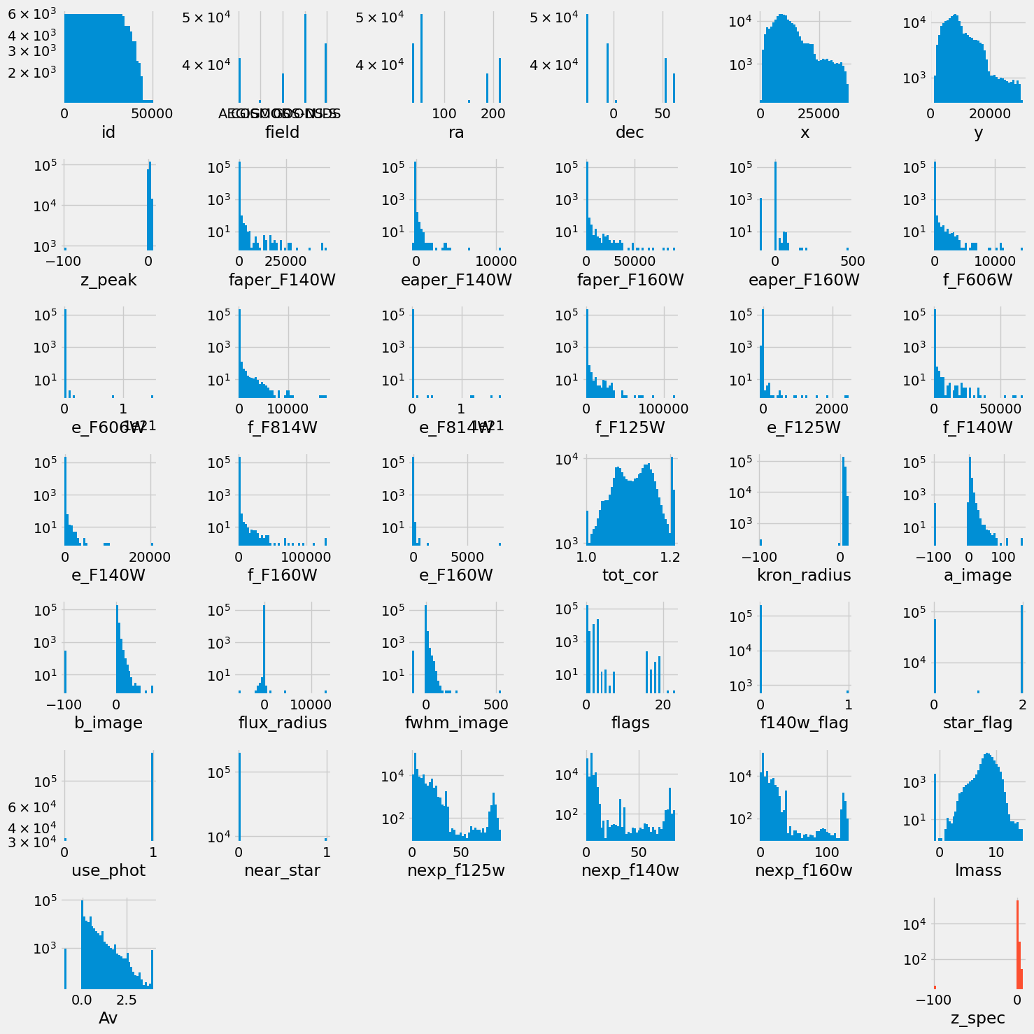
df.describe().TIn the following, we plot the distribution of all the columns.
columns = [k for k in df.columns if k != "z_spec"]
wrap = 6  # number of columns to show in a row
nlines = (len(columns) + 1) // wrap + int((len(columns) + 1) % wrap > 0)
fig, axs = plt.subplots(nlines, wrap, figsize=(15, 15))
for i, ax in enumerate(axs.ravel()):
    if i >= len(columns):
        ax.axis("off")
        continue
    ax.hist(df[columns[i]], bins=43, log=True)
    ax.set_xlabel(columns[i])

ax = axs[-1, -1]
ax.axis("on")
plt.hist(df["z_spec"], bins=43, log=True, color="C1")
plt.xlabel("z_spec")
plt.tight_layout()

Markdown("""
> Distribution of all the columns in our dataset before feature selection and any preprocessing.
""")
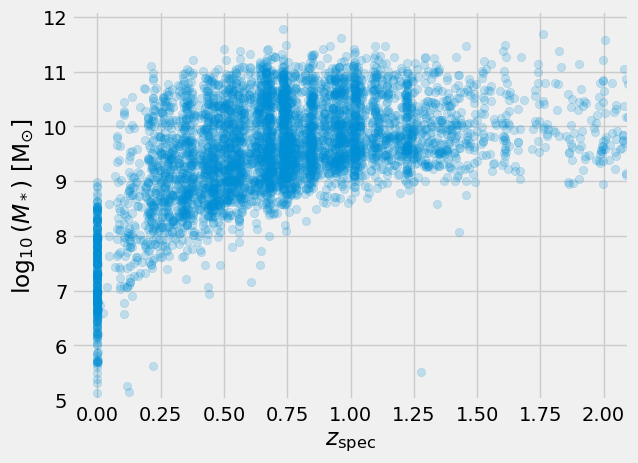
We are astronomers, we can therefore consider physical relationships between the features. For example, mass vs. redshift
ax = plt.subplot(111)

ax.scatter(df.z_spec, df.lmass, alpha=0.2)
ax.set_xlabel(r"$z_{\rm spec}$")
ax.set_ylabel(r"$\log_{10}{(M_*)}$ [M$_{\odot}$]")
ax.set_xlim(-0.1, 2.1)
ax.set_ylim(5.0, 12.1)
display(
    Markdown("""
> Physical parameters mass vs. redshift.
We find a pileup of redshit estimates at 0 and even negative estimates. In addition, some
masses are negative. These need to be cleaned for further uses.
""")
)
What do we conclude from this exploration?
Before building and applying a regression model, we have to deal with
negative
z_specvaluesbad values (-99.0) in flux measurements
Data cleaning, Feature selection, and Data leakage
We need to deal with bad/missing values, and select the features we will use to predict the redshift.
Feature selection & data leakage
Definition: Data leakage is when information about the label takes part into the training dataset to create the model. This additional information can allow the model to learn or know something that it otherwise would not know and in turn invalidate the estimated performance of the mode being constructed.
For example, if z_peak, lmass or z_spec remain in the training features. Sometimes it could be suddle: for instance including a MonthlySalary column when predicting YearlySalary; or MinutesLate when predicting if a train will be late.
Data leakage can cause you to create overly optimistic if not completely invalid predictive models.
We do not keep
z_phot,z_peak, andlmassto avoid leakage.The
Av,lmassandz_peakvalues come from the FAST photometric fit, and so we will exclude them as well.We will exclude the categorical flag variables (
flags,f140w_flag,star_flag,use_phot,near_star). To first order redshift estimates should be driven by the flux values. We remove the flags to reduce the feature space. We can check if they help later on.
remove = (
    "Av",
    "lmass",
    "z_peak",
    "flags",
    "f140w_flag",
    "star_flag",
    "use_phot",
    "near_star",
    "z_spec",
    "id",
    "field",
    "ra",
    "dec",
    "x",
    "y",
)

# we define the features from the remaining columns and the target is the spectroscopic redshift
features = [col for col in df.columns if col not in remove]
target = "z_spec"

Markdown(f"""
**features** {features}

**target**: {target} """)Value filtering and imputing missing values
We need to curate the dataset to remove bad objects and values. Here “bad” remains to be defined. Depending on the features we select, we may need to transform text fields into values/categories.
Look at the selected data and see if some values are strange, missing, etc. Is there a regime where the redshift will be difficult to learn?
OneHot encoder / categorical values
The example below shows how to proceed. (Note that we did not decide to keep flags in this notebook)
# Using sklearn to encode labels
from sklearn.preprocessing import LabelEncoder
df['field_lbl'] = LabelEncoder().fit_transform(df['field'])
Pandas can also encode the labels into categories (Categorical type). This is useful when we have a column with text values that we want to convert into numerical values.
df['field_lbl] = df['field'].astype('category').cat.codesFiltering out / curating the dataset
By inspecting the datset, we find that some filtering is necessary.
By inspection of mass vs redshift, we will only keep sources with to remove sources that do not have complete coverage across redshift.
We will also remove redshift value = 0, which likely corresponds to a star.
And we remove redshift <= 0. Negative values are bad estimates.
# target = z_spec defined above
df = df.loc[(df['lmass'] > 9) & (df[target] > 0)].copy()note:
df[(df['lmass'] > 9) & (df[target] > 0)] is a boolean “mask” that selects the rows that satisfy the conditions and creates a view / slice of the initial dataframe. This can lead to issues if we modify the slice. To avoid this, we can use .copy() which makes a copy of the slice.
Imputing missing values
We need to take care of the missing or bad values.
In linear regression problems, the least informative alteration is to use the median or mean of the distribution. In presence of outliers, median would be more robust.
In the following, we use the median of the distributions to replace bad / missing values, i.e flux mesurements = -99.0.
# inpute missing data in all column names ending with 'W' (e.g. f160w, e_f160w, eaper_f140w, etc.)
ecols = [col for col in features if col.endswith("W")]
ecols
['faper_F140W',
'eaper_F140W',
'faper_F160W',
'eaper_F160W',
'f_F606W',
'e_F606W',
'f_F814W',
'e_F814W',
'f_F125W',
'e_F125W',
'f_F140W',
'e_F140W',
'f_F160W',
'e_F160W']for col in ecols:
missing_value = np.nanmedian(df[col])
df[col] = df[col].fillna(missing_value)
df.loc[df[col] < -90, col] = missing_valueFinal dataset
df_x = df[features]
df_y = df[target]
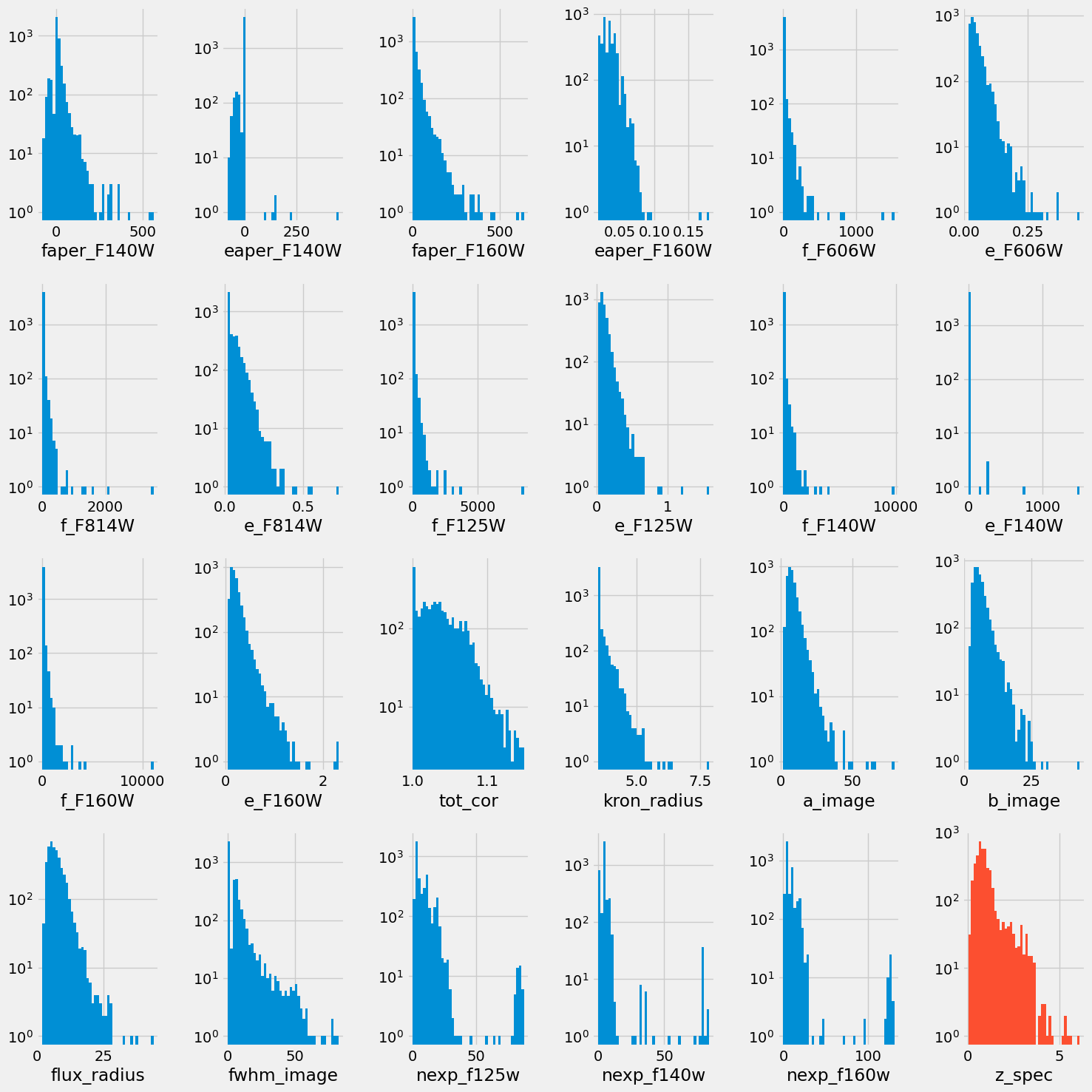
print("The final data set contains {0:,d} samples and {1:,d} features".format(len(df_x), len(df_x.columns)))The final data set contains 4,173 samples and 23 features
columns = [k for k in df_x.columns]
wrap = 6  # number of columns to show in a row
nlines = (len(columns) + 1) // wrap + int((len(columns) + 1) % wrap > 0)
fig, axs = plt.subplots(nlines, wrap, figsize=(15, 15))
for i, ax in enumerate(axs.ravel()):
    if i >= len(columns):
        ax.axis("off")
        continue
    ax.hist(df_x[columns[i]], bins=43, log=True)
    ax.set_xlabel(columns[i])

ax = axs[-1, -1]
ax.axis("on")
plt.hist(df_y, bins=43, log=True, color="C1")
plt.xlabel("z_spec")
plt.tight_layout()

Markdown("""
> Distribution of all the feature columns we selected and the target (red) after preprocessing.
""")
As we are about to make a linear regression model, we can look into the correlations between all the features and z_spec as below.
plt.figure(figsize=(5, 8))
corr = df_x.corrwith(df_y, method="spearman")
corr = corr.sort_values()
plt.barh(np.arange(len(corr)), corr, tick_label=corr.index)
plt.title("Spearman correlation with z_spec")
Markdown(
    """> Spearman correlation of the selected features and the target spectroscopic redshift."""
)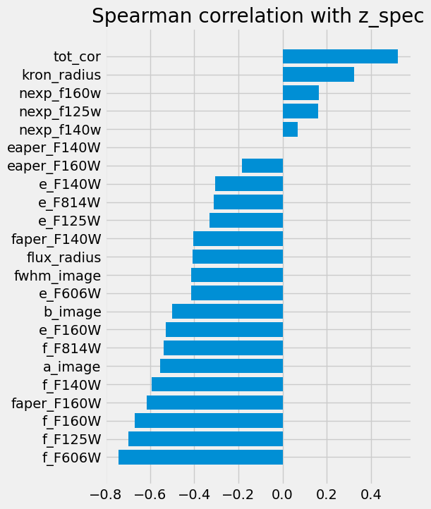
These correlations make sense:
the width of a source indicates that we see the host galaxy, hence a low-redshift source.
the fluxes link to the photometric redshift, which is when the various lines move from the blue bands to the redder ones. ...
Building a regression model
In this part, we will use the scikit-learn library to build a linear regression model.
(see scikit-learn documentation
In the next part of the workshop, we will explore models based on neural networks.
What is machine learning?
In its essence, Machine learning refers to the ability of computer systems to automatically learn and improve from experience without explicit programming. We attribute the foundation of machine learning to Arthur Samuel (see image) who tought a computer how to play checkers in 1959 and to Tom Mitchell who gave it the modern spin in 1997: Machine Learning is the study of computer algorithm that allow computer programs to automatically improve through experience.
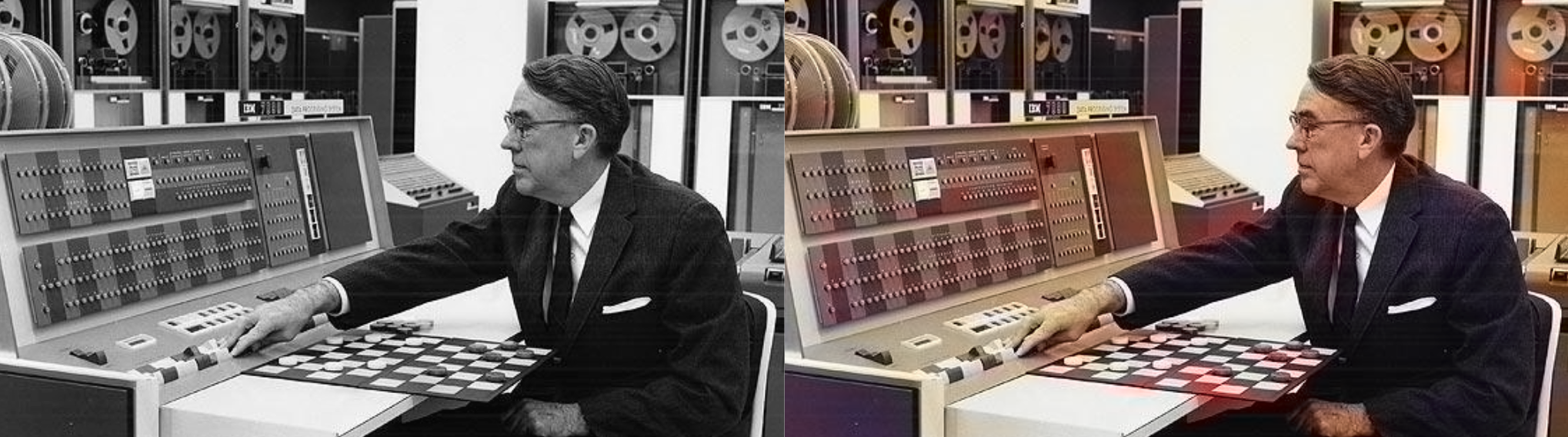
“Field of study that gives computers the ability to learn without being explicitly programmed.” Arthur Samuel, Teaching a computer to play checkers, 1959 Left is the original black and white image. Right the image processed to infer colors using ML algorithm (colorize-it.com).
Machine learning is part of the grand scheme of automated machine decisions. In computer science, a rule-based system is a system that stores and manipulate knowledge to interpret information or take decisions in a useful way. Normally, the term rule-based system only applies to systems involving human-crafted or curated rule sets. For instance in a factory, if an item is not conforming to the size or shape rule, it will be discarded.
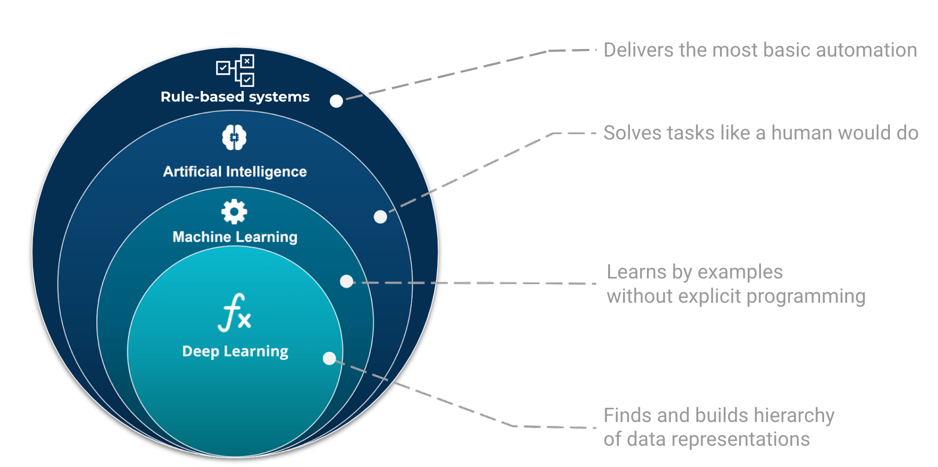
The place and role of AI, ML, and Deep Learning in automated machine decisions. Image adapted from Tukijaaliwa, CC BY-SA 4.0, via Wikimedia Commons, original source
If those sets of rules are not explicitly programmed but learned, we enter the domain of artificial intelligence, e.g. automatic rule inference. Artificial intelligence is broad and aims at tackling problems the way humans do. For example, evolutionary algorithms are a family of optimization algorithms inspired by processes of natural evolution. They help to solve complex optimization problems by iteratively improving a population of candidate solutions over multiple generations.
Finally, we have a category of algorithms that can learn from examples. One could see this category as a family of algorithms that update their code (or parameters) based on a learning process.
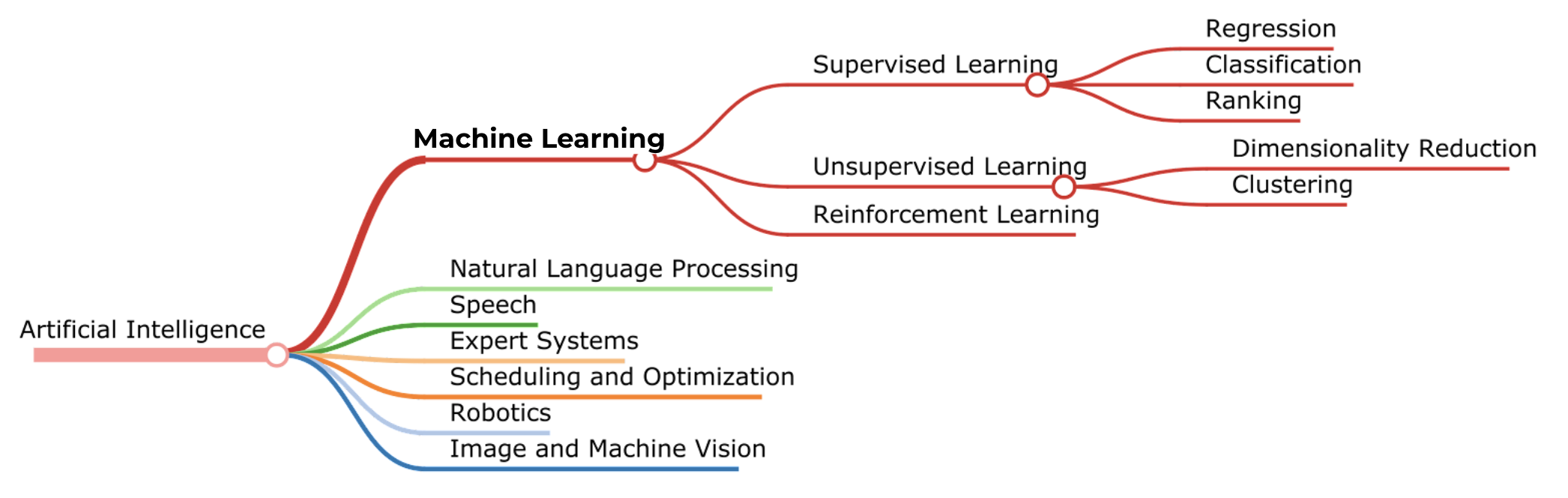
Machine learning is only one branch of AI and the learning processes are commonly divided into three categories: supervised, unsupervised, and reinforced learning. Deep learning is a subpart of the machine learning family.
💡 Summary ML is a “Field of non-trivial data analysis of complicated data sets”
ML involves
data description, interpretation
prediction
inference, i.e. learning from the data
ML Algorithms
can extract information from high dimensional data
find general properties, structures of the data
we can map those properties to physical interpretation
⚠️ Machine learning is NOT A “~magical~ universal analysis of complicated data sets”
ML does not provide
data compilation, and understanding
scientific interpretation
critical thinking
ML Algorithms
Should never remain a black box
Will always return “an” answer
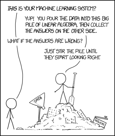
Machine learning is the intersection of computer science and mathematics and lacks domain expertise required to properly interpret the outputs. - image source: xkcd
Scikit learn: a machine learning library for Python
Scikit-learn is a free software machine learning library for the Python programming language. It features various classification, regression, and clustering algorithms including support vector machines, random forests, gradient boosting, k-means, and DBSCAN.
The library itself follows the tree structure above, but also provides tools to preprocess data and analyze the predictions.
Here we explore a few options for regressor models. You can find all available models on the sklearn documentation.
One particular convenience of sklearn is its standard API for any model. You can test almost anything with four steps:
from sklearn.<path> import Modelmodel = Model(**parameters), whereparameterswill vary from model type to model type.model.fit(X, y), the actual training step whereXis the features andythe target.ypred = model.predict(X)
We will start with a simple linear regression model.
from sklearn.linear_model import LinearRegressionBut first we need to understand the concepts and proper practice for training a model.
Concept of training a model
In machine learning, we train a model to learn the relationship between the features and the target variable. The model is trained on a training dataset. The model is then used to make predictions on new data.
In machine learning the training set matters gianormously to make our models accurate and performant. To understand it better, I always use the elephant parable:
Six blind persons are asked to describe an elephant by touching its body parts. A first one feels its side and describes it as a wall, a second touches its tusk and thinks it is a spear, a third one feels the trunk and confidently identifies a snake, a fourth touches a knee and believes it could be a tree, the fifth palps the ear and thinks of a fan and, finally, a sixth holds the tail and assumes the elephant is a rope.
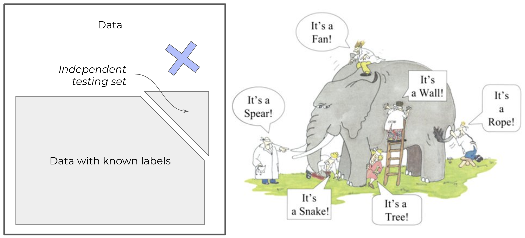
None of the blind people was wrong in their analysis. They plausibly described what they touched and felt. The challenge comes from their limited perception. They each assumed their interaction was representative of the full picture, but they were wrong.
This parable represents exactly what training sets do to machine learning. But often it could be hard to know it’s an elephant, we don’t always have the whole picture to check.
The training set must be sufficiently representative of the whole picture to lead to the right conclusion. If any of the blind people would cross check with another, their conclusions would most likely be different.
Validating: the “Generalization problem”
How do we know if our model is good? We need to validate it on a validation dataset that was not used to train the model. This is called validation.
Validation is an essential step when developing a machine learning model as it ensures that the training set accurately represents what will happen during application deployment. To validate a machine learning model, one should mask part of their training set and use this blind test on their trained algorithm or neural network before deploying into production environment . It’s also important for validation sets not only contain representative elements but also unseen elements so as to properly assess how well your system can adapt given new inputs and scenarios which may occur during its applications.
Validating and testing your algorithms with unseen data helps ensure we created an accurate representation of reality and that we identify any potential issues before they become critical errors down the line.
At its core, validating ML Model is testing and understanding the limits of our system’s ability at adapting given new input parameters while still maintaining accuracy throughout all possible scenarios within our application domain. This adaptation is a generalization problem.
💡 Training, testing, applying: the three inevitable ones
Training: Giving (labeled or unlabeled) data to your method and letting it find a mapping between input and output variables.
Testing: Using a new piece of data to check the mapping works outside the training. Determines performance of the model.
Applying: Applying to a dataset that is neither trained or tested on, for which the “correct” answer is unknown.
Generalizing: Enabling applications to other “domains” (e.g. extrapolating).
from sklearn.model_selection import train_test_split

# first reserve 70% of the data for training, 30% for validation
X_train, X_validate, y_train, y_validate = train_test_split(
    df_x, df_y, test_size=0.3, random_state=42
)

# second, split the validation set in half to obtain validation and test sets.
X_validate, X_test, y_validate, y_test = train_test_split(
    X_validate, y_validate, test_size=0.5, random_state=42
)
Note that sklearn plays nice with Pandas dataframes, so we can directly use the df dataframe we created earlier. The splitting of the data preserves the indices and structure of the dataframe(s).
X_trainLinear Regression Model
Let’s do a simple one first
from sklearn.linear_model import LinearRegression

lin = LinearRegression()
lin.fit(X_train, y_train)How do we quantify the performance of our model?
To quantify the performance of the model, we will apply it to the validation set and compare the predicted values with the true values by computing the mean squared error (MSE). Again sklear has you covered!
from sklearn.metrics import mean_squared_errorfrom sklearn.metrics import mean_squared_error
y_predict = lin.predict(X_test)
y_predict0 = lin.predict(X_train)
mse = mean_squared_error(y_test, y_predict)
fig, ax = plt.subplots(1, 1, figsize=(4, 4))
ax.scatter(y_test, y_predict, alpha=0.2, label="test")
ax.scatter(y_train, y_predict0, alpha=0.2, label="train", zorder=-1)
ax.plot(ax.get_xlim(), ax.get_xlim(), zorder=-1, color="0.5")
ax.set_aspect("equal")
ax.set_xlim(-0.1, 5)
ax.set_ylim(-0.1, 5)
ax.grid()
ax.set_xlabel("Truth (y_test)")
ax.set_ylabel("Prediction (y_predict)")
plt.legend(loc="upper left")
ax.text(0.9, 0.9, f"MSE={mse:0.4f}", transform=ax.transAxes, ha="right")
Markdown(f"""
> The prediction of the redshifts using a linear regression model. The model is not very good, the MSE = {mse:.4f}, but it's a start.
We can see that the model is not very good at predicting redshifts, especially for high redshifts where the bias is significant.""")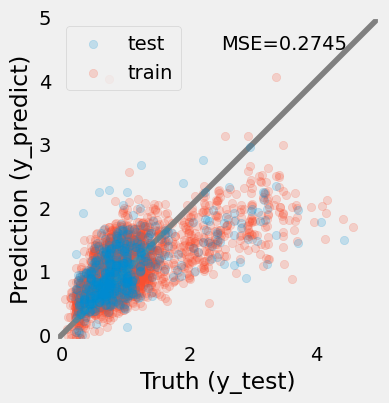
This plot shows that the linear regression model is getting the bulk of the data but performs poorly when the data becomes sparse, i.e. .
How do we know which features drive the prediction?
We can look at the coefficients of each feature from the model using the LinearRegression.coef_ attribute.
importances = lin.coef_
labels = lin.feature_names_in_
# older version: labels = df_x.columns
argsort = np.argsort(importances)
fig, ax = plt.subplots(1, 1, figsize=[10, 10])
ax.barh(
    np.arange(len(df_x.columns)),
    importances[argsort],
    align="center",
    height=0.5,
    tick_label=labels,
)
ax.set_xlabel("Lin. Coeffs")
Markdown(""" > Coefficients of the linear model sorted by values.""")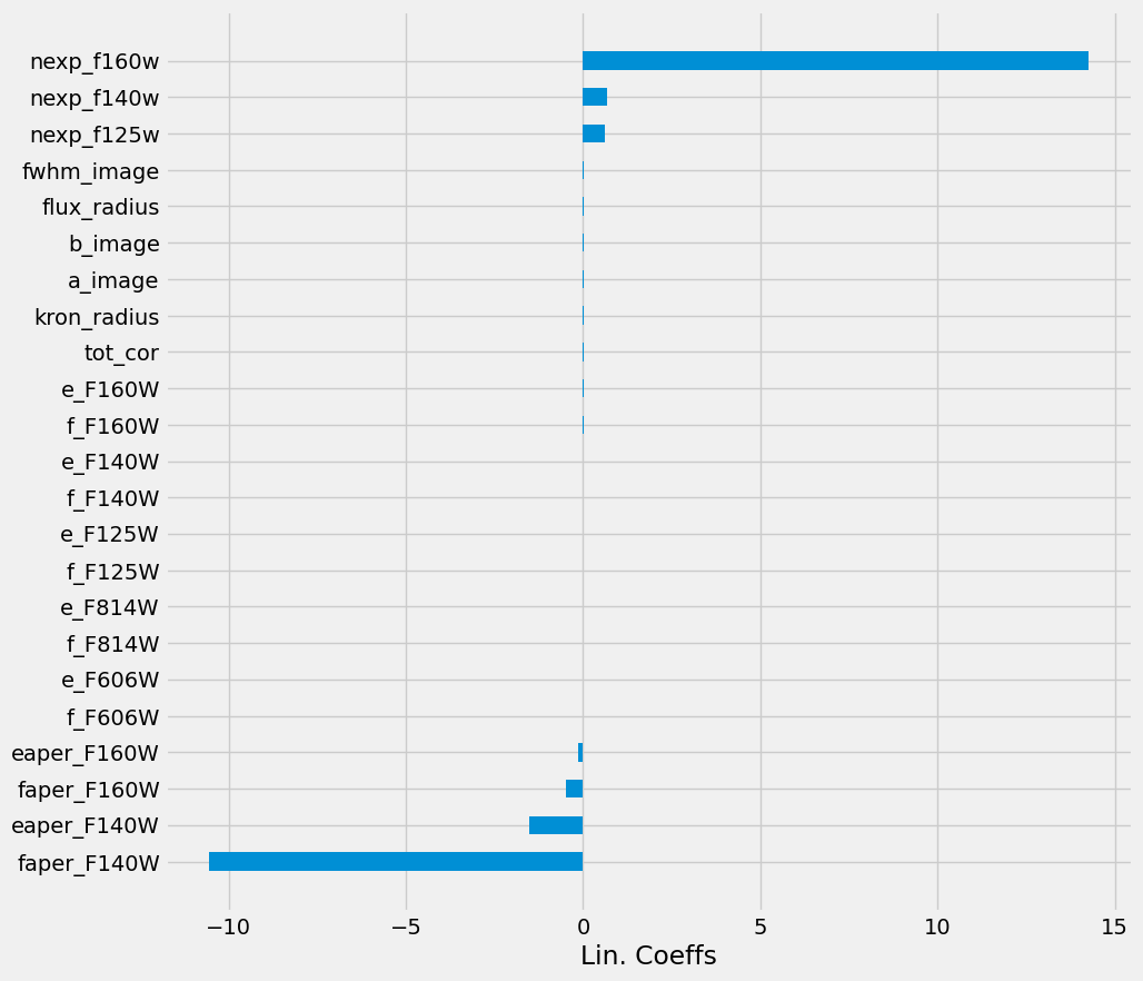
However, note here that we have features with very different dynamical ranges. Hence comparing feature amplitudes does not reflect how important these are for the model. One would need to normalize the dimensions first. (We do so in the next model.)
Overall the MSE is not great. Not surprising given the simplicity of our model. Maybe we can do better by changing it?
What simple model could we try next?
Polynomial regression model
In this section, we explore a polynomial model. Such a model takes an input feature vector and turns it into for a degree=2 polynomial.
see sklearn.preprocessing.PolynomialFeatures
To make this modeling more robust, we will also normalize the data. We will use
see sklearn.preprocessing.StandardScaler
We will also switch from a traditional linear regression to a regularized regression. This regularization is one or multiple additional terms in the loss function that penalizes the number of non-null coefficients.
see for example: sklearn.linear_model.LassoLars, sklearn.linear_model.ElasticNet
In the following we use sklearn.linear_model.LassoLarsIC, a lasso model fit with Lars using BIC or AIC for model selection (setting how strong the penalization should be).
Our training flow is then:
We first create the polynomial features
We then normalize the data
We fit the model
And we need to keep track of our transformations to apply them to the validation set (or any new data). Luckily, sklearn has a Pipeline object that chains transformations and models.
from sklearn.pipeline import Pipelinefrom sklearn.pipeline import Pipeline
from sklearn.preprocessing import PolynomialFeatures, StandardScaler
from sklearn.linear_model import LassoLarsIC
pipe = Pipeline(
[
("polynomial", PolynomialFeatures(degree=2)),
("scaler", StandardScaler()),
("classifier", LassoLarsIC()),
]
)
pipe.fit(X_train, y_train)In the above, we also use Pipeline, which is a convenient wrapper around sequential steps:
here, we expand X_train to a polynomial of degree=2, then standardize the data before applying the regressor. Pipeline is an object that understands the API and knows which functions to call for each step.
Manually, the pipe.fit would be something like
Xprime = polynomial.fit_transform(X_train)
Xscaled = scaler.fit_transform(Xprime)
classifier.fit(X_train, y_train)
Then to predict values, similar steps would be necessary
Xprime = polynomial.transform(X_test)
Xscaled = scaler.fit_transform(Xprime)
ypred = classifier.fit(X_test, y_test)
but pipe.predict is more convenient.
How does the model perform?
# This is the same code as above
y_predict = pipe.predict(X_test)
y_predict0 = pipe.predict(X_train)
mse = mean_squared_error(y_test, y_predict)

fig, ax = plt.subplots(1, 1, figsize=(4, 4))
ax.scatter(y_test, y_predict, alpha=0.2, label="test")
ax.scatter(y_train, y_predict0, alpha=0.2, label="train", zorder=-1)
ax.plot(ax.get_xlim(), ax.get_xlim(), zorder=-1, color="0.5")
ax.set_aspect("equal")
ax.set_xlim(-0.1, 5)
ax.set_ylim(-0.1, 5)
ax.grid()
ax.set_xlabel("Truth (y_test)")
ax.set_ylabel("Prediction (y_predict)")
plt.legend(loc="best")
ax.text(0.9, 0.9, f"MSE={mse:0.4f}", transform=ax.transAxes, ha="right")
Markdown(f"""
> The prediction of the redshifts using a polynomial regression model (degree={pipe['polynomial'].degree}). The model is still not very good, the MSE = {mse:.4f}.
The bias at high redshits remains significant.""")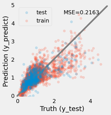
The results look better (MSE shows ~20% improvement). The looks closer to the identity line, but still not perfect.
Which features are important?
pipe['classifier'].coef_importances = pipe["classifier"].coef_
labels = pipe["polynomial"].get_feature_names_out()
# older version: labels = df_x.columns
argsort = np.argsort(np.abs(importances)) # absolute importance
show_n = 10
argsort = argsort[-show_n:]
importances = importances[argsort]
labels = labels[argsort]
argsort = np.argsort(importances) # for aesthetic
plt.figure()
ax = plt.subplot(111)
ax.barh(
np.arange(len(labels)),
importances[argsort],
align="center",
height=0.5,
tick_label=labels[argsort],
)
ax.set_xlabel("Normalized Coeffs")
Markdown(
""" > Coefficients of the polynomial model sorted by absolute values. The regularization has set many of the coefficients to zero that we do not represent here."""
)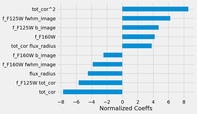
Interestingly, the model selected features that are fluxes multiplied by full-width-half-maximum (fwhm) of the image. This is not totally surprising as the fwhm is a proxy for the size of the source, which is a proxy for the redshift.
The residuals of our linear regression models are not great. We can explore other kinds of models. Changing the degree of the polynomial could help, or the regularization. Eventually, linear models do not seem to be the best fit for this problem.
Using sklearn, we can easily test different models. In particular, we can use non-linear ones.
Exploring models
Random Forest
Using sklearn, we can very easily construct a decision tree model for regressing redshift from the photometric catalog features. A decision tree is composed of a series of if-else decision steps. The number of steps and the types of decision at each step is determined by training the algorithm with supervision. In this first example, we will use the DecisionTreeRegressor from sklearn.
from sklearn.ensemble import RandomForestRegressorfrom sklearn.ensemble import RandomForestRegressor
# use the same parameters as the Decision Tree
# Initialize the model
rf = RandomForestRegressor()
rf.fit(X_train, y_train)y_predict = rf.predict(X_test)
y_predict0 = rf.predict(X_train)
mse = mean_squared_error(y_test, y_predict)
fig, ax = plt.subplots(1, 1, figsize=(4, 4))
ax.scatter(y_test, y_predict, alpha=0.2, label="test")
ax.scatter(y_train, y_predict0, alpha=0.2, label="train", zorder=-1)
ax.plot(ax.get_xlim(), ax.get_xlim(), zorder=-1, color="0.5")
ax.set_aspect("equal")
ax.set_xlim(-0.1, 5)
ax.set_ylim(-0.1, 5)
ax.set_xlabel("Truth (y_test)")
ax.set_ylabel("Prediction (y_predict)")
plt.legend(loc="best")
ax.text(0.9, 0.9, f"MSE={mse:0.4f}", transform=ax.transAxes, ha="right")
Markdown(f"""
> The prediction of the redshifts using a random forest model . The model improves significantly compared with the previous attemps, MSE = {mse:.4f}.
The bias at high redshits may remains but it is significantly reduced.""")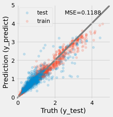
The results are much improved by the random forest!
However, we must be cautious. It is possible that this model suffers from over-fitting.
Bias, Variance, Over-fitting, and Under-fitting
Overfitting is a common problem in machine learning, where a model learns the detail and noise in the training data to the extent that it negatively impacts the performance of the model on new data. This means that the noise or random fluctuations in the training data is picked up and learned as concepts by the model. The problem is that these concepts do not apply to new data and negatively impact the models ability to generalize.
x = np.logspace(0, 1, 8)
ytrue = (x / 10) ** 2
y = ytrue + np.random.randn(len(x)) * 0.05
plt.plot(x, ytrue, "k", ls="--", alpha=0.5, lw=2, label="Truth")
plt.plot(x, y, "ko", zorder=100)

x_eval = np.linspace(x.min(), x.max(), 100)
for degree in [1, 2, 10]:
    poly = PolynomialFeatures(degree=degree)
    X = poly.fit_transform(x[:, None])
    X_eval = poly.transform(x_eval[:, None])
    preds = LinearRegression().fit(X, y).predict(X_eval)
    plt.plot(x_eval, preds, label=f"d={degree}")
plt.xlabel("x")
plt.ylabel("y")
plt.ylim(-0.15, 1.3)
plt.legend()

Markdown(
    """ > Example of under/over-fitting using polynomial regression with different degrees. The model with degree 2 is underfitting, and degree 10 is overfitting the data."""
)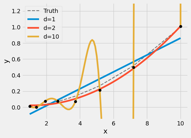
In the above figure, we see polynomial fits for three different degrees .
, the model underfit, the model is too simplistic, and overall predictions will be inaccurate. This model suffers from bias. The reason for this label is that the model makes strong assumptions about the form of the underlying function that maps inputs to outputs.
, the model overfit, the model is too flexible (has too many free parameters) it can pass through the training data perfectly. But any new data will be terribly predicted. This model suffers from high variance: any small update of one will lead to an extremely different model.
, the model is just right (duh!). It captures the underlying trend of the data, but is not too flexible. This model has a good balance between bias and variance.
To visualize overfitting, we can compare the mean squared error (MSE) for models of increasing max_depth on the training and testing sets.
💡 Lucky for us that our model here is fast to train. In some cases, exploring values for the model’s parameters can become extremely expensive.
# Implementation that shows an example of
# parallel processing with joblib (installed with sklearn)
from joblib import delayed, Parallel


def compute_mse(max_depth, X_train, y_train, X_test, y_test):
    params = {
        "min_samples_split": 15,
        "min_samples_leaf": 5,
    }
    rf = RandomForestRegressor(max_depth=max_depth, **params)
    rf.fit(X_train, y_train)

    y_predict_train = rf.predict(X_train)
    y_predict_test = rf.predict(X_test)

    mse_values = (
        max_depth,
        mean_squared_error(y_train, y_predict_train),
        mean_squared_error(y_test, y_predict_test),
    )
    return mse_values


max_depths = np.arange(1, 20, 2).astype(int)

results = Parallel(n_jobs=-1)(
    delayed(compute_mse)(depth, X_train, y_train, X_test, y_test)
    for depth in max_depths
)
results = np.array(results)
fig, ax = plt.subplots(1, 1)
ax.plot(results[:, 0], results[:, 1], color="blue", label="Training Set")
ax.plot(results[:, 0], results[:, 2], color="orange", label="Test Set")
final_interval = results[:, 0] >= 10.0
ax.hlines(
[results[final_interval, 1].mean()],
xmin=results[:, 0].min(),
xmax=results[:, 0].max(),
color="blue",
alpha=0.5,
linestyle="--",
lw=2,
)
ax.hlines(
[results[final_interval, 2].mean()],
xmin=results[:, 0].min(),
xmax=results[:, 0].max(),
color="orange",
alpha=0.5,
linestyle="--",
lw=2,
)
ax.set_xlabel("max depth")
ax.set_ylabel("MSE")
ax.legend()
Markdown("""
> The MSE for the training and test sets as a function of the maximum depth of the trees in the random forest model.
The model is overfitting for depths greater than 10, as the test error diverges from the train error.
At low depths, the model is underfitting, and the error is high for both sets.""")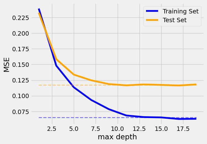
Beyond a max_depth of ~10, the MSE on the training set declines while the MSE on the test set flattens out, suggesting some amount of over-fitting: the flattening indicates that the model does not learn anything more from the data, so we can stop the complexity early.
Note that sometimes, the residuals could increase again on the test set.
Cross-validation
To explore further, we will explore how general our model performance (here quantifed with MSE) is using k-fold cross-validation via sklearn. In practice, the X and y datasets are split into k “folds”, and over k iterations, the model is trained using k-1 folds as training data and the remaining fold as a test set to compute performace (i.e., MSE).
from sklearn.model_selection import cross_validatefrom sklearn.model_selection import cross_validate
cv = cross_validate(
estimator=rf,
X=df_x,
y=df_y,
cv=5, # number of folds
scoring="neg_mean_squared_error",
n_jobs=-1,
)
print(
f'Cross-validated MSE score: {-cv["test_score"].mean():.3f} +/- {cv["test_score"].std():.3f}'
)Cross-validated MSE score: 0.139 +/- 0.051
💡 We used the full data set with known labels because the cross-validation procedure sets a train and test set at every fold.
The previous MSE is consistent with the cross-validated MSE, suggesting that the model is not significantly over-fitting.
Feature importance
Next, we’ll observe which features are most important to the model predictions. Note that as trees implements selections per dimensions, a normalization of the data is not necessary.
# plot we did before
importances = rf.feature_importances_
argsort = np.argsort(importances)
fig = plt.figure(figsize=[10, 10])
ax = fig.add_subplot(111)
ax.barh(
    np.arange(len(df_x.columns)),
    importances[argsort],
    align="center",
    height=0.5,
    tick_label=np.array(features)[argsort],
)
ax.set_xlabel("Feature importance");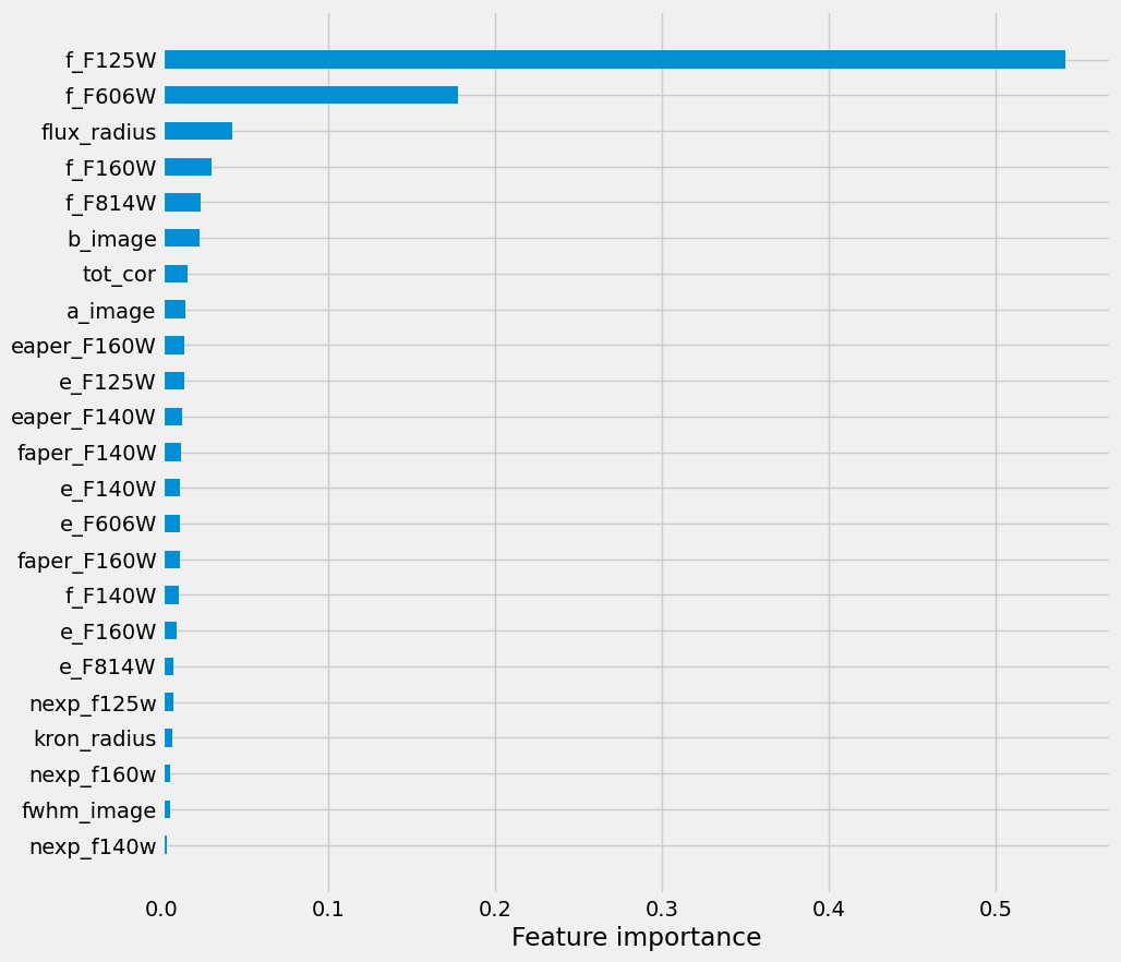
We see that basically our model is by a few bands (F606, F814W, F160W, F125W) and the width of the aperture.
⚠️ Warning: the feature importance in trees is not robust due to the manner they are build (see also sklearn documentation). In practice, these are indicative, but if you need a proper characterization, you will need something like the SHAP values (SHapley Additive exPlanations), e.g. SHAP package.
import shap

shap_values = shap.TreeExplainer(rf).shap_values(X_train)
shap.summary_plot(shap_values, X_train, plot_type="bar")
import matplotlib.pyplot as plt

f = plt.figure()
shap.summary_plot(shap_values, X_train)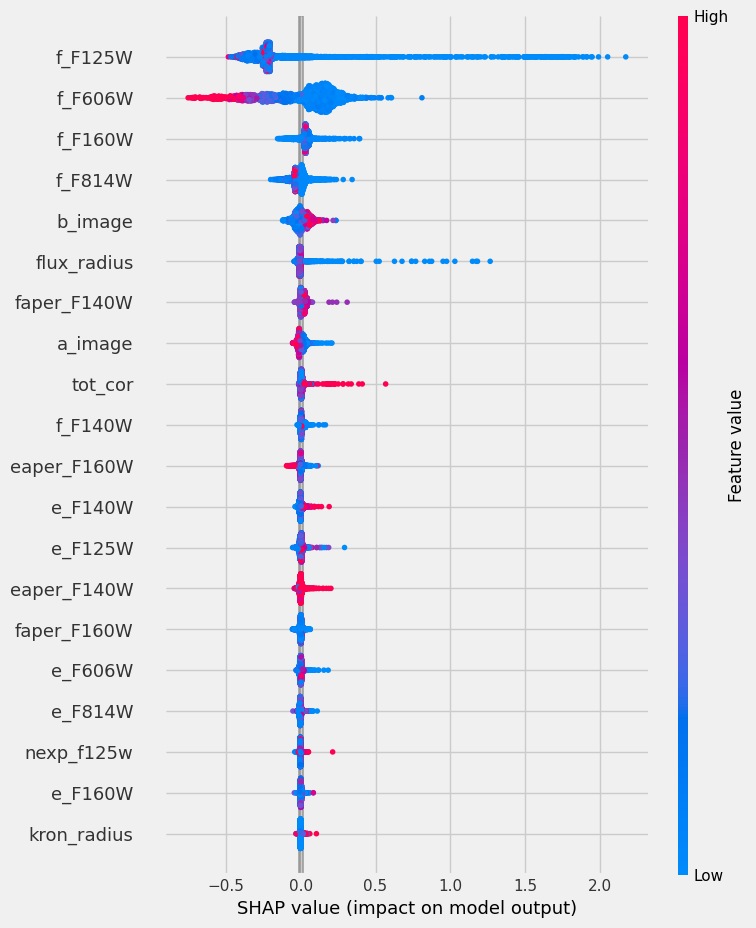
SHAP values are expensive to compute, these are equivalent to a leave-one-out procedure on each feature. However, they also provide more insight into what information pieces are relevant to the model.
Other models
In this section, we explore any interesting model that sklearn provides (e.g. lighGBM, HistGradientBoostingRegressor). We will train the models and compare their performance based on the root-MSE metric and diagnostic plots.
from sklearn.ensemble import HistGradientBoostingRegressor


et = HistGradientBoostingRegressor()
et.fit(X_train, y_train)

pipe2 = Pipeline(
    [
        ("polynomial", PolynomialFeatures(degree=2)),
        ("scaler", StandardScaler()),
        ("classifier", HistGradientBoostingRegressor()),
    ]
)

pipe2.fit(X_train, y_train);
from sklearn.metrics import root_mean_squared_error
y_values = [
lin.predict(X_validate),
pipe.predict(X_validate),
rf.predict(X_validate),
et.predict(X_validate),
pipe2.predict(X_validate),
df["z_peak"].loc[X_validate.index],
]
yp_train = [
lin.predict(X_train),
pipe.predict(X_train),
rf.predict(X_train),
et.predict(X_train),
pipe2.predict(X_train),
df["z_peak"].loc[X_train.index],
]
names = [
"linear",
"polynomial",
"random forest",
"lightGBM",
"poly+lightGBM",
"Skelton et al. 2014",
]
fig, ax = plt.subplots(2, len(names) // 2, figsize=(10, 10))
for k, (ax, ypt, yval) in enumerate(zip(np.ravel(ax), yp_train, y_values)):
color = None
if k == len(names) - 1:
color = "C3"
ax.scatter(y_train, ypt, alpha=0.2, color=color)
ax.scatter(y_validate, yval, alpha=0.2, color=color)
ax.set_aspect("equal")
ax.set_xlim(-0.1, 5)
ax.set_ylim(-0.1, 5)
ax.plot(ax.get_xlim(), ax.get_xlim(), zorder=-1, color="0.5")
ax.set_xlabel("Truth (z_spec)")
ax.set_ylabel("prediction (y_predict)")
ax.set_title(names[k])
mse = root_mean_squared_error(y_validate, yval)
ax.text(0.01, 0.9, f"RMSE = {mse:.4f}", transform=ax.transAxes)
ax = plt.gcf().get_axes()[-1].set_ylabel("prediction (z_peak)")
plt.tight_layout()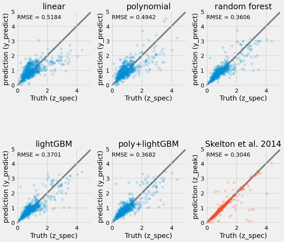
Going further
What if you include galaxy colors (e.g., F125W-F140W, F140W-F160W, F606W-F125W)? do the model results improve? Can you think of other features to include?
Can you tune the model parameters with a grid search?
What if you try other models from sklearn?
- Skelton, R. E., Whitaker, K. E., Momcheva, I. G., Brammer, G. B., van Dokkum, P. G., Labbé, I., Franx, M., van der Wel, A., Bezanson, R., Da Cunha, E., Fumagalli, M., Förster Schreiber, N., Kriek, M., Leja, J., Lundgren, B. F., Magee, D., Marchesini, D., Maseda, M. V., Nelson, E. J., … Wuyts, S. (2014). 3D-HST WFC3-SELECTED PHOTOMETRIC CATALOGS IN THE FIVE CANDELS/3D-HST FIELDS: PHOTOMETRY, PHOTOMETRIC REDSHIFTS, AND STELLAR MASSES. The Astrophysical Journal Supplement Series, 214(2), 24. 10.1088/0067-0049/214/2/24
- Skelton, R. E., Whitaker, K. E., Momcheva, I. G., Brammer, G. B., van Dokkum, P. G., Labbé, I., Franx, M., van der Wel, A., Bezanson, R., Da Cunha, E., Fumagalli, M., Förster Schreiber, N., Kriek, M., Leja, J., Lundgren, B. F., Magee, D., Marchesini, D., Maseda, M. V., Nelson, E. J., … Wuyts, S. (2014). 3D-HST WFC3-SELECTED PHOTOMETRIC CATALOGS IN THE FIVE CANDELS/3D-HST FIELDS: PHOTOMETRY, PHOTOMETRIC REDSHIFTS, AND STELLAR MASSES. The Astrophysical Journal Supplement Series, 214(2), 24. 10.1088/0067-0049/214/2/24