Some Fun with Numba

This is a notebook to demonstrate numba following this article: https://pythonspeed.com/articles/numba-faster-python/

The example is a simple function which takes an array and calculates the monotonically increasing version:

[1, 2, 1, 3, 3, 5, 4, 6] → [1, 2, 2, 3, 3, 5, 5, 6]

#!pip install numpy
#!pip install numba

import numpy as np
from numba import njit

Let’s create a function that does the work we need

# Defining a regular function
def monotonically_increasing(a):
     max_val = 0
     for i in range(len(a)):
         if a[i] > max_val:
             max_val = a[i]
         a[i] = max_val
     return a

# Defining the numba decorated function
@njit
def numba_monotonically_increasing(a):
     max_val = 0
     for i in range(len(a)):
         if a[i] > max_val:
             max_val = a[i]
         a[i] = max_val
     return a

Tip

you can use result = %timeit -o to record the execution time

# Let's check performance
# First run regular function:
time_numpy_1 = %timeit -o monotonically_increasing(np.random.randint(0, 1000000, 1000000))

142 ms ± 571 µs per loop (mean ± std. dev. of 7 runs, 10 loops each)

# Second run regular function:
time_numpy_2 = %timeit -o monotonically_increasing(np.random.randint(0, 1000000, 1000000))

141 ms ± 462 µs per loop (mean ± std. dev. of 7 runs, 10 loops each)

# Third run regular function:
time_numpy_3 = %timeit -o monotonically_increasing(np.random.randint(0, 1000000, 1000000))

140 ms ± 909 µs per loop (mean ± std. dev. of 7 runs, 10 loops each)

Duration of execution is the same.

# First run numba function:
time_numba_1 = %timeit -o numba_monotonically_increasing(np.random.randint(0, 1000000, 1000000))

4.34 ms ± 30.4 µs per loop (mean ± std. dev. of 7 runs, 1 loop each)

# Second run numba function:
time_numba_2 = %timeit -o numba_monotonically_increasing(np.random.randint(0, 1000000, 1000000))

4.33 ms ± 12.8 µs per loop (mean ± std. dev. of 7 runs, 100 loops each)

# Third run numba function:
time_numba_3 = %timeit -o numba_monotonically_increasing(np.random.randint(0, 1000000, 1000000))

4.33 ms ± 10.7 µs per loop (mean ± std. dev. of 7 runs, 100 loops each)

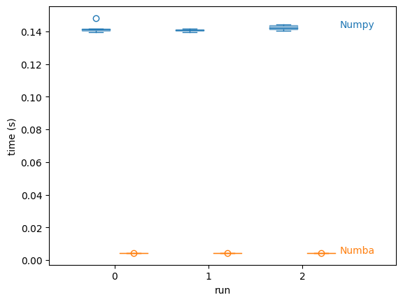
First run is much slower (function is compiled) but subsequent runs are ~14 times faster!

Woah! For a sample run the first took 162 ms, while the second took 4.5 seconds on average.

264/9.64

27.38589211618257

~27 times faster!!!

Note: the actual execution times will vary depending on the underlying system and the type of problem you are solving.

import matplotlib.pyplot as plt

# plot times from timeit outputs
data = [run.timings for run in (time_numpy_1, time_numpy_2, time_numpy_3)]
pos = np.arange(len(data))
c = 'C0'
plt.boxplot(data, positions=pos - 0.2, 
            patch_artist=True,
            boxprops=dict(facecolor=c, color=c, alpha=0.5),
            capprops=dict(color=c),
            whiskerprops=dict(color=c),
            flierprops=dict(color=c, markeredgecolor=c),
            medianprops=dict(color=c))
plt.text(pos[-1] + 0.4, np.mean(data[-1]), f'Numpy',
         color=c, weight='roman', ha='left')

data = [run.timings for run in (time_numba_1, time_numba_2, time_numba_3)]
pos = np.arange(len(data))
c = 'C1'
plt.boxplot(data, positions=pos + 0.2, 
            patch_artist=True,
            boxprops=dict(facecolor=c, color=c, alpha=0.5),
            capprops=dict(color=c),
            whiskerprops=dict(color=c),
            flierprops=dict(color=c, markeredgecolor=c),
            medianprops=dict(color=c))

plt.text(pos[-1] + 0.4, np.mean(data[-1]), f'Numba',
         color=c, weight='roman', ha='left')

plt.xlim(plt.xlim()[0], plt.xlim()[1] + 0.3)
plt.xticks(pos, pos)
plt.ylabel('time (s)')
plt.xlabel('run');